palaeoclimate – Cabot Institute for the Environment blog

Learning lessons from the past to inform the future

Posted on August 24, 2020April 4, 2023 by janet.crompton

A fairly recent blog post on the EGU blog site reiterated the compelling comparison between the current COVID-19 crisis and the ongoing climate emergency, focusing on extreme events such as hurricanes, heatwaves and severe rainfall-related flooding, all of which are likely to get worse as the climate warms (Langendijk & Osman 2020). This comparison has been made by us Climate Scientists since the COVID-19 crisis began; both the virus and the disastrous impacts of anthropogenic climate change were (and indeed are) predictable but little was done in the ways of preparedness, both were (and are still being) underestimated by those in power despite warnings from science, and both are global in extent and therefore require united action. Another comparison is that both are being intensively, and urgently, researched across the world by many centres of excellence. We don’t have all the answers yet for either, but progress is being made on both.

When it comes to understanding our climate, there are several approaches; these are, of course, not mutually exclusive. We can focus on present-day climate variability, to understand the physical mechanisms behind our current climate; examples include, but are not limited to, ocean-atmosphere interactions, land-atmosphere feedbacks, or extreme events (see Williams et al. 2008, Williams & Kniveton 2012 or Williams et al. 2012, as well as work from many others).

Alternatively, we can use our current understanding of the physical mechanisms driving current climate to make projections of the future, either globally or regionally. State-of-the-art General Circulation Models (GCMs) can provide projections of future climate under various scenarios of socio-economic development, including but not limited to greenhouse gas (GHG) emissions (Williams 2017).

A third approach is to focus on climates during the deep (i.e. geological) past, using tools to determine past climate such as ice cores, tree rings and carbon dating. Unlike the historical period, which usually includes the past in which there are human observations or documents, the deep past usually refers to the prehistoric era and includes timescales ranging from thousands of years ago (ka) to millions of years ago (Ma). Understanding past climate changes and mechanisms is highly important in improving our projections of possible future climate change (e.g. Haywood et al. 2016, Otto-Bliesner et al. 2017, Kageyama et al. 2018, and many others).

One reason for looking at the deep past is that it provides an opportunity to use our GCMs to simulate climate scenarios very different to today, and compare these to scenarios based on past.

These days I am primarily focusing on the latter approach, and am involved in almost all of the palaeoclimate scenarios coming out of UK’s physical climate model, called HadGEM3-GC3.1. These focus on different times in the past, such as the mid-Holocene (MH, ~6 ka), the Last Glacial Maximum (LGM, ~26.5 ka), the Last Interglacial (LIG, ~127 ka), the mid-Pliocene Warm Period (Pliocene, ~3.3 Ma) and the Early Eocene Climate Optimum / Paleocene-Eocene Thermal Maximum (EECO / PETM, collectively referred to here as the Eocene, ~50-55 Ma). All of these have been (or are being) conducted under the auspices of the 6th phase of the Coupled Modelling Intercomparison Project (CMIP6) and 4th phase of the Palaeoclimate Modelling Intercomparison Project (PMIP4).

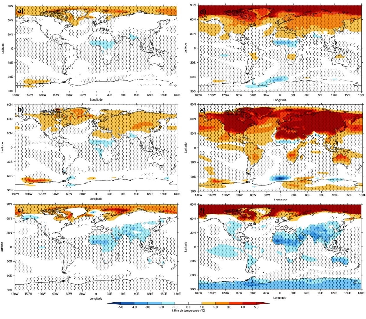
Figure 1: Calendar adjusted 1.5 m air temperature climatology differences, mid-Holocene and last interglacial simulations from the UK’s physical climate model, relative to the preindustrial era: a-c) mid Holocene – preindustrial; d-f) last interglacial – preindustrial. Top row: Annual; Middle row: Northern Hemisphere summer (June-August); Bottom row: Northern Hemisphere winter (December-February). Stippling shows statistical significance (as calculated by a Student’s T-test) at the 99% level. Taken from Williams et al. (2020).

These five periods are of particular interest to the above projects for a number of different reasons. Before these are discussed, however, the fundamentals of deep past climate change need to be briefly introduced. In short, climate changes in the geological past (i.e. without human influence) can either be internal to the planet (e.g. volcanic eruptions, oceanic CO2 release) or external to the planet (e.g. changes in the Earth’s orbit around the Sun). Arguably, it is changes to the amount of incoming solar radiation (known as insolation) that is the primary driver behind all long-term climate change. Theories for long-term climate change, such as the beginning and ending of ice ages, began to be proposed during the 1800s. However, it wasn’t until 1913 that the Serbian mathematician, Milutin Milankovitch, developed our modern day understanding of glacial cycles. In short, Milankovitch identified three interacting cycles concerning the Earth’s position relative to the Sun: a) Eccentricity, in which the Earth’s orbit around the Sun changes from being more or less circular on a period of 100-400 ka; b) Obliquity, in which the Earth’s axis changes from being more or less tilted towards the Sun on a period of ~41 ka; and c) Precession, in which the Earth’s polar regions appear to ‘wobble’ around the axis (like a spinning top coming to its end) on a period of ~19-24 ka. All of these three cycles not only change the overall amount of insolation received by the planet, and therefore its average temperature, but also where the most energy is received; this ultimately determines the strength and timing of our seasons.

With this background in mind, and returning to the paleoclimate scenarios mentioned above, the MH and the LIG collectively represent a ‘warm climate’ state. During these periods the Earth’s axis was tilted slightly more towards the Sun, resulting in an increase in Northern Hemisphere insolation (because of the larger landmasses here relative to the Southern Hemisphere). This caused much warmer Northern Hemisphere summers and enhanced African, Asian and South American monsoons (Kageyama et al. 2018). The increase in temperatures can be seen in Figure 1, where clearly the largest increases relative to the preindustrial era (PI) are in the Northern Hemisphere during June-August (Williams et al. 2020). By comparing model simulations to palaeoclimate reconstructions during these periods, the models’ ability to simulate these climates can be tested and this therefore assesses our confidence in future projections of climate change; which, as mentioned above, may result in more rainfall extremes and enhanced monsoons.

In contrast, the LGM represents a ‘cold climate’ state which, although unlikely to return as a result of increasing anthropogenic GHG emissions, nevertheless provides a well-documented climatic period during which to test the models. Going back further in time, the Pliocene is the most recent time in the geological past when CO2 levels were roughly equivalent to today, and was a time when global annual mean temperatures were 1.8-3.6°C higher than today (Haywood et al. 2016). See Figure 2 for the increases in sea surface temperature (SST) during the Pliocene, relative to today. This annual mean temperature increase is clearly much higher than the current target, as specified by the Paris Agreement, of keeping warming below 1.5°C (at most 2°C) by the end of 2100. Importantly, the CO2 increases and subsequent warming during the Pliocene occurred over timescales of thousands to millions of years, whereas anthropogenic GHG emissions have caused a similar increase in CO2 (from ~280 parts per million (ppmv) during the PI to just over 400 ppmv today) in under 300 years. The Pliocene, therefore, provides an excellent analogy for what our climate might be like in the (possibly near) future.

Finally, going back even further, the Eocene is the most recent time in the past that was characterised by very high CO2 concentrations, twice or more than that of today at >800-1000 ppmv; this resulted in temperatures ~5°C higher than today in the tropics and ~20°C higher than today at high latitudes (Lunt et al. 2012, Lunt et al. 2017). The reason the Eocene is highly relevant, and of concern, is that these CO2 concentrations are roughly equivalent to those projected to occur by the end of 2100, if the Representative Concentration Pathway (RCP) 8.5 scenario, also known as the ‘Business-as-usual’ scenario, which was used in the most recent IPCC report (IPCC 2014), becomes reality. The Eocene, therefore, provides an excellent albeit concerning analogy for what the worse-case scenario could be like in the future, if action is not taken.

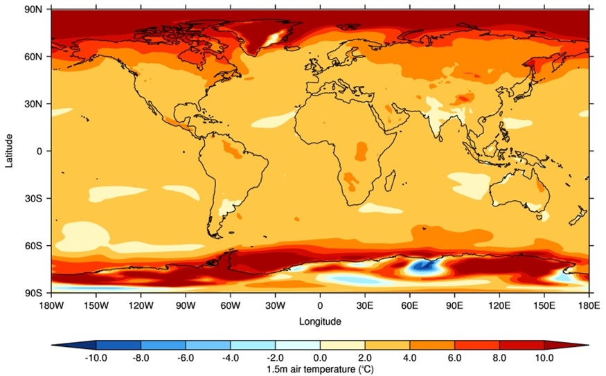
Figure 2: 1.5 m air temperature climatology differences, Pliocene simulation from the UK’s physical climate model, relative to the preindustrial era.

Understanding the climate, how it has changed in the past and how it might change in the future is a complex task and subject to various interrelated approaches. One of these approaches, the concept of using the past to inform the future (e.g. Braconnot et al. 2011), has been described here. Just like in the case of COVID-19, it is our responsibility as Climate Scientists to work together across approaches and disciplines, as well as reliably communicating the science to governments, policymakers and the general public, in order to mitigate the crisis as much as possible.

References

Braconnot, P., Harrison, S. P., Otto-Bliesner, B, et al. (2011). ‘The palaeoclimate modelling intercomparison project contribution to CMIP5’. CLIVAR Exchanges Newsletter. 56: 15-19

Haywood, A. M., Dowsett, H. J., Dolan, A. M. et al. (2016). ‘The Pliocene Model Intercomparison Project (PlioMIP) Phase 2: scientific objectives and experimental design’. Climate of the Past. 12: 663-675

IPCC (2014). ‘Climate Change 2014: Synthesis Report. Contribution of Working Groups I, II and III to the Fifth Assessment Report of the Intergovernmental Panel on Climate Change’ [Core Writing Team, R.K. Pachauri and L.A. Meyer (eds.)]. IPCC. Geneva, Switzerland, 151 pp

Kageyama, M., Braconnot, P., Harrison, S. P. et al. (2018). ‘The PMIP4 contribution to CMIP6 – Part 1: Overview and over-arching analysis plan’. Geoscientific Model Development. 11: 1033-1057

Langendijk, G. S. & Osman, M. (2020). ‘Hurricane COVID-19: What can COVID-19 tell us about tackling climate change?’. EGU Blogs: Climate. https://blogs.egu.eu/divisions/cl/2020/04/16/corona-2/. Accessed 24/7/20

Lunt, D. J., Dunkley-Jones, T., Heinemann, M. et al. (2012). ‘A model–data comparison for a multi-model ensemble of early Eocene atmosphere–ocean simulations: EoMIP’. Climate of the Past. 8: 1717-1736

Lunt, D. J., Huber, M., Anagnostou, E. et al. (2017). ‘The DeepMIP contribution to PMIP4: experimental design for model simulations of the EECO, PETM, and pre-PETM (version 1.0)’. Geoscientific Model Development. 10: 889-901

Otto-Bliesner, B. L., Braconnot, P., Harrison, S. P. et al. (2017). ‘The PMIP4 contribution to CMIP6 – Part 2: Two interglacials, scientific objective and experimental design for Holocene and Last Interglacial simulations’. Geoscientific Model Development. 10: 3979-4003

Williams, C. J. R., Kniveton, D. R. & Layberry, R. (2008). ‘Influence of South Atlantic sea surface temperatures on rainfall variability and extremes over southern Africa’. Journal of Climate. 21: 6498-6520

Williams, C. J. R., Allan, R. P. & Kniveton, D. R. (2012). ‘Diagnosing atmosphere-land feedbacks in CMIP5 climate models’. Environmental Research Letters. 7 (4)

Williams, C. J. R. & Kniveton, D. R. (2012). ‘Atmosphere-land surface interactions and their influence on extreme rainfall and potential abrupt climate change over southern Africa’. Climatic Change. 112 (3-4): 981-996

Williams, C. J. R. (2017). ‘Climate change in Chile: an analysis of state-of-the-art observations, satellite-derived estimates and climate model simulations’. Journal of Earth Science & Climatic Change. 8 (5): 1-11

Williams, C. J. R., Guarino, M-V., Capron, E. (2020). ‘CMIP6/PMIP4 simulations of the mid-Holocene and Last Interglacial using HadGEM3: comparison to the pre-industrial era, previous model versions, and proxy data’. Climate of the Past. Accepted

——————————–

This blog was written by Cabot Institute member Dr Charles Williams, a climate scientist within the School of Geographical Sciences, University of Bristol. His research focusses on deep time to understand how climate has behaved in the warmer worlds experienced during the early Eocene and mid-Pliocene (ca. 50 – 3 Mio years ago). This blog was reposted with kind permission from Charles. View the original blog on the EGU blog site.

Dr Charles Williams

How ancient warm periods can help predict future climate change

Posted on April 26, 2016April 6, 2023 by janet.crompton

Several more decades of increased carbon dioxide emissions could lead to melting ice sheets, mass extinctions and extreme weather becoming the norm. We can’t yet be certain of the exact impacts, but we can look to the past to predict the future.

We could start with the last time Earth experienced CO₂ levels comparable to those expected in the near future, a period 56m to 34m years ago known as the Eocene.

The Eocene began as a period of extreme warmth around 10m years after the final dinosaurs died. Alligators lived in the Canadian Arctic while palm trees grew along the East Antarctic coastline. Over time, the planet gradually cooled, until the Eocene was brought to a close with the formation of a large ice sheet on Antarctica.

During the Eocene, carbon dioxide (CO₂) concentrations in the atmosphere were much higher than today, with estimates usually ranging between 700 and 1,400 parts per million (ppm). As these values are similar to those anticipated by the end of this century (420 to 935ppm), scientists are increasingly using the Eocene to help predict future climate change.

We’re particularly interested in the link between carbon dioxide levels and global temperature, often referred to as “equilibrium climate sensitivity” – the temperature change that results from a doubling of atmospheric CO₂, once fast climate feedbacks (such as water vapour, clouds and sea ice) have had time to act.

To investigate climate sensitivity during the Eocene we generated new estimates of CO₂ throughout the period. Our study, written with colleagues from the Universities of Bristol, Cardiff and Southampton, is published in Nature.

Reconstruction of the 40m year old planktonic foraminifer Acarinina mcgowrani.
Richard Bizley (www.bizleyart.com) and Paul Pearson, Cardiff University, CC BY

As we can’t directly measure the Eocene’s carbon dioxide levels, we have to use “proxies” preserved within sedimentary rocks. Our study utilises planktonic foraminifera, tiny marine organisms which record the chemical composition of seawater in their shells. From these fossils we can figure out the acidity level of the ocean they lived in, which is in turn affected by the concentration of atmospheric CO₂.

We found that CO₂ levels approximately halved during the Eocene, from around 1,400ppm to roughly 770ppm, which explains most of the sea surface cooling that occurred during the period. This supports previously unsubstantiated theories that carbon dioxide was responsible for the extreme warmth of the early Eocene and that its decline was responsible for the subsequent cooling.

We then estimated global mean temperatures during the Eocene (again from proxies such as fossilised leaves or marine microfossils) and accounted for changes in vegetation, the position of the continents, and the lack of ice sheets. This yields a climate sensitivity value of 2.1°C to 4.6°C per doubling of CO₂. This is similar to that predicted for our own warm future (1.5 to 4.5°C per doubling of CO₂).
Our work reinforces previous findings which looked at sensitivity in more recent time intervals. It also gives us confidence that our Eocene-like future is well mapped out by current climate models.

Fossil foraminifera from Tanzania – their intricate shells capture details of the ocean 33-50m years ago.
Paul Pearson, Cardiff University, CC BY

Rich Pancost, a paleoclimate expert and co-author on both studies, explains: “Most importantly, the collective research into Earth history reveals that the climate can and has changed. And consequently, there is little doubt from our history that transforming fossil carbon underground into carbon dioxide in the air – as we are doing today – will significantly affect the climate we experience for the foreseeable future.”

Our work also has implications for other elements of the climate system. Specifically, what is the impact of higher CO₂ and a warmer climate upon the water cycle? A recent study investigating environmental change during the early Eocene – the warmest interval of the past 65m years – found an increase in global precipitation and evaporation rates and an increase in heat transport from the equator to the poles. The latter is consistent with leaf fossil evidence from the Arctic which suggests that high precipitation rates were common.

However, changes in the water cycle are likely to vary between regions. For example, low to mid latitudes likely became drier overall, but with more intense, seasonal rainfall events. Although very few studies have investigated the water cycle of the Eocene, understanding how this operates during past warm climates could provide insights into the mechanisms which will govern future changes.

———————–
This blog was written by Cabot Institute member Gordon Inglis, Postdoctoral Research Associate in Organic Geochemistry, University of Bristol and Eleni Anagnostou, Postdoctoral Research Fellow, Ocean and Earth Science, University of Southampton

This article was originally published on The Conversation. Read the original article.

Setting-up new collaborations with geoscientists from Kazakhstan

Posted on March 20, 2014April 19, 2023 by janet.crompton

A map of Kazakstan
(from GraphicMaps.com, World Atlas)

Landlocked in central Asia, Kazakhstan is the world 9th largest country, larger than Western Europe. It is host to one of largest amounts of accessible minerals and fossil fuel. Even though, Kazakhstan is relatively unknown to the general public and geoscientists. In order to encourage international research collaboration between ambitious young researchers from the UK and Kazakhstan, in March 2014 the British Council Researcher Links organized a workshop in Ust-Kamenogorsk in Kazakhstan.

I was selected to attend this meeting and as a result I found myself on a Monday afternoon boarding a plane to Kazakhstan together with 12 other UK scientists. My main reason to attend the workshop was that palaeoclimatic reconstructions from this part of the world are almost non-existant. This while in the geological past (Mesozoic and Paleogene) Kazakhstan was on the bottom of a large epicontinental ocean that connected the Tethys Ocean with the Arctic. Any palaeoclimatic records from this region of the world are thus very valuable and could provide key-insights into deep-time paleoclimate. I hoped that some scientists worked on palaeoclimate reconstructions. Publications were sparse, and sometimes in Russian, so hopefully a face-to-face meeting would be good start for collaboration.

The modern campus of the East Kazakhstan
State Technical University in Ust-Kamenogorsk.

The first personal encounter with the vast size of Kazakhstan and remoteness was the time in took us to get there. Flying from London, it took us more than 24 hours to get to the small city of Ust-Kamenogorsk, located in northeastern Kazakhstan. Although temperatures in the UK reached a comfortable 18 degrees C that day, in Ust-Kamenogorsk day temperatures were well below freezing and winter still in full swing. Snow was packed half a meter high at the side of the roads.

The workshop was held at the modern campus of the East Kazakhstan State Technical University. The first days were filled with presentations from both UK and Kazakh scientists, as well as Simon Williams, the Director of the British Council Kazakhstan. An interpreter was used to translate Russian into English and vice versa. It was very interesting to give a presentation with an interpreter, it makes you very conscious of what you say and forces you to talk in brief and concise sentences. I was very happy to hear that several Kazakh palaeoclimatologist were present and very enthusiastic to share their results and ideas. Although palaeoclimate is not a top research priority in Kazakhstan, it was impressive to see the work that was already done. Several scientists worked on sections covering all periods from the Cambrian to the early Cenozoic and detailed stratigraphies were developed. We saw dinosaur eggs, beautifully preserved fossil leaves, fossil fish, and remains of large ferns. Very exciting! We had an impressive lab tour in which they showed us an array of state-of-the-art instruments that would make some UK-geoscientists jealous.

All geared-up and ready to descend into the mine.

(I am on the right!)

As a main theme of the workshop was mining, the 3^rd day we visited the Maleevka Mine near Zyryanovsk. After a detailed explanation of the daily operations of the mine, which mainly produces copper and zinc, we went down into the mine and had an amazing and slick two-hour tour. Although I am not an expert in mining, it was fascinating to see the mining operations from close-by. I was impressed by the state-of-the-art technology and know-how and safety regulations.

Remote-controlled mine dozer used to safely
get ore from newly blasted areas.

After four intense days (and nights), it was time to make the 30hr journey back to Bristol. My overall impression is that Kazakhstan is an amazingly beautiful country. It was impressive to fly for hours over snow-covered steppe and mountains. Although the weather was cold, the people were incredible warm and friendly. Wherever we went, people welcomed us with smiles and food, lots and lots of great food! The workshop was incredibly well organized. I definitely want to come back to this country. In fact, the last day one scientist gave me some Paleocene samples that I literally had to smuggle out of the country and which we will use for a pilot study. In the near future we aim to organize another workshop in Kazakhstan, focusing especially on palaeoclimate and hopefully some fieldwork because there is so much potential for great science and collaboration!

The British Council organized this trip. The UK coordinator was Prof. K. Jeffrey from the Camborne School of Mines, University of Exeter.

This blog is written by Dr David Naafs who is a Postdoctoral Research Fellow in the Organic Geochemistry Research Unit at the Cabot Institute, University of Bristol.

AGU 2013: The importance of 400 ppm CO2

Posted on February 11, 2014April 19, 2023 by janet.crompton

On 1 June 2012, a concentration of 400 ppm carbon dioxide was measured in air samples in the Arctic. On 9 May 2013, Mauna Loa, the longest recording station, measured a daily average of 400 ppm carbon dioxide. Next year we may see the global average concentration reach 400 ppm and the year after that 400 ppm could be measured at the South Pole. The 400 ppm number is arbitrary, but it is a symbol of the anthropogenic climate change that scientists have been talking about for many years.

Here at the University of Bristol, the upcoming 400 ppm epoch prompted the question of what do we know about 400 ppm CO2 climates and how could it be used to galvanize action on climate change? But 400 ppm and climate change is a bigger issue than one University can take on, so we took our idea to the American Geosciences Union Fall conference. With more than 24,000 attendees each year, AGU is the perfect place to talk about what 400 ppm CO2 means in a scientific sense and what we as scientists should do about communicating it.

Two sessions were proposed: one looking at the science of 400 ppm CO2 climates, co-convened with Kerim Nisanciouglu of the University of Bergen, Norway, the other at communicating 400 ppm co-convened with Kent Peacock of University of Lethbridge and Casey Brown of UMass Amherst.

Naomi Oreskes (pictured) asked why scientists
don’t allow themselves to sound alarmed when reporting alarming conclusions from their
research.

The communication session looked at how climate science could be communicated effectively. First to speak was Naomi Oreskes, who asked why scientists don’t allow ourselves to sound alarmed when we’re reporting alarming conclusions. Citing from neuroscience research, Oreskes argued that when scientists conform to the ‘unemotional scientist’ paradigm they actually risk being less rational and sounding inauthentic. It was clear that Oreskes’ points struck the audience, as many of them queued up to ask questions.

Myles Allen made a compelling case for sequestered adequate fraction of extracted (SAFE) carbon – i.e. compulsory carbon capture and storage. Allen pointed out that people will always pay to burn carbon and argued that a carbon price is just a way to ‘cook the planet slower’. Robert Lempert took a less controversial stand and explained how uncertainty can be managed in robust decision making. Using hydrological examples, Lempert suggested that by starting with the desired outcome and working backwards, uncertainty can be dealt with. The session finished with James Hansen, talking about the right message, and how the things that people care about needs to be communicated by the best communicators. Criticising the pursuit of unconventional fossil fuels, Hansen argued the need for a carbon tax which was redistributed back to people. A lively question and answer session followed, with all the speakers engaging in a strong discussion and the audience contributing pointed questions. No problems with talking without emotion in this session!

The 400 ppm physical science session started by focussing on what information we could draw from climates in the past where CO2 is believed to have been ~400 ppm. The first speaker was Alan Haywood who summarised the work of the PlioMIP project which tries to understand the climate of the Pliocene (~3 million years ago) – what it was like and why. The Pliocene is the most recent time period in the past when atmospheric CO2 concentrations could have been as high as they are today. Two more Pliocene presentations followed. First, Natalie Burls (standing in for Chris Brierley) explained that even with CO2 set to 400 ppm in their climate model simulations they could not match the warm temperatures reconstructed by Pliocene data – suggesting that either the climate models are not sensitive enough to CO2 or that there are other dynamical processes that we do not fully understand yet. Thomas Chalk gave a comparison between different methods for reconstructing CO2 in the past, and concluded that the Pliocene concentration was indeed at around 400 ppm. The final talk in the palaeoclimate part of the session was given by Dana Royer who presented the most compelling evidence for very different climates in the past with polar forests at 80°N indicating annual mean temperatures in the Arctic that were 30°C warmer than they are today! Dana presented new CO2 reconstructions demonstrating that the CO2 concentration at the time of the polar forests could have been around 400 ppm, again suggesting that our climate models may not be sensitive enough to CO2.

The next part of the session looked at current CO2 levels with a presentation by Steven Davis about the amount of CO2 that we have already committed to putting into the atmosphere. The energy infrastructure that we have already built amounts to future CO2 emissions of 318Gt, and new global commitments are still increasing. Vaughan Pratt followed with a talk about the reasons for the recent pause in the global warming trend, separating out natural causes and anthropogenic causes using mathematical and statistical analyses. He concludes that the recent pause is of natural origin.

The final part of the session peered through the looking glass into the future. Andrew Friedman investigates the causes of the temperature asymmetry between the northern hemisphere and the southern hemisphere and how that asymmetry may alter under the future climate emission scenarios. He concluded that the asymmetry is set to increase into the next century, with the northern hemisphere warming faster than the southern hemisphere and projects that the tropical rainbelt will shift northwards as a result.

Kirsten Zickfield has found that warming in the next
millenium might amount to 1 degree globally,
concentrated at the Poles. Sea levels are projected to
rise by 0.8m.

The final talk of the session was given by Kirsten Zickfeld who examined the climate changes we might already be committed to as a result of the CO2 emissions we have already released (under the assumption that atmospheric CO2 stays at 400 ppm). She used a climate model with biogeochemical components to identify how long it would take for the climate to reach equilibrium with the present CO2 concentration of 400 ppm, what the climatic impacts of that equilibrium might be and whether it might be possible to return to CO2 levels below 400 ppm on human timescales by using negative emissions (carbon capture/storage schemes). She found that the already committed warming into the next millennium might amount to 1°C globally, concentrated at the poles. Sea levels are projected to rise by 0.8m due to thermal expansion alone and further increases of 10m due to ice melt are possible over much longer timescales. Committed changes for the ‘other CO2 problem’ – ocean acidification – are relatively small, with a pH drop of only 0.01 projected. She concludes that even if CO2 levels could drop below 400 ppm in the future, whilst air temperatures may stabilise, sea level may continue to rise due to thermal expansion alone.

Both of the sessions were recorded for access after the event and provoked a lot of debate, during the sessions and online. We hope that in some small way these sessions have helped scientists think differently about what 400 ppm means and what we can do about it.

This blog was written by T Davies-Barnard and Catherine Bradshaw, Geographical Sciences, University of Bristol.