ice sheet – Cabot Institute for the Environment blog

Arctic is warming nearly four times faster than the rest of the world – new research

Posted on August 16, 2022April 16, 2023 by janet.crompton

New research estimates that the Arctic may be warming four times faster than the rest of the world.
Netta Arobas/Shutterstock

The Earth is approximately 1.1℃ warmer than it was at the start of the industrial revolution. That warming has not been uniform, with some regions warming at a far greater pace. One such region is the Arctic.

A new study shows that the Arctic has warmed nearly four times faster than the rest of the world over the past 43 years. This means the Arctic is on average around 3℃ warmer than it was in 1980.

This is alarming, because the Arctic contains sensitive and delicately balanced climate components that, if pushed too hard, will respond with global consequences.

Why is the Arctic warming so much faster?

A large part of the explanation relates to sea ice. This is a thin layer (typically one metre to five metres thick) of sea water that freezes in winter and partially melts in the summer.

The sea ice is covered in a bright layer of snow which reflects around 85% of incoming solar radiation back out to space. The opposite occurs in the open ocean. As the darkest natural surface on the planet, the ocean absorbs 90% of solar radiation.

When covered with sea ice, the Arctic Ocean acts like a large reflective blanket, reducing the absorption of solar radiation. As the sea ice melts, absorption rates increase, resulting in a positive feedback loop where the rapid pace of ocean warming further amplifies sea ice melt, contributing to even faster ocean warming.

This feedback loop is largely responsible for what is known as Arctic amplification, and is the explanation for why the Arctic is warming so much more than the rest of the planet.

Blocks of melting sea ice revealing a deep blue sea. — Melting sea ice in the Arctic Ocean.
Nightman1965/Shutterstock

Is Arctic amplification underestimated?

Numerical climate models have been used to quantify the magnitude of Arctic amplification. They typically estimate the amplification ratio to be about 2.5, meaning the Arctic is warming 2.5 times faster than the global average. Based on the observational record of surface temperatures over the last 43 years, the new study estimates the Arctic amplification rate to be about four.

Rarely do the climate models obtain values as high that. This suggests the models may not fully capture the complete feedback loops responsible for Arctic amplification and may, as a consequence, underestimate future Arctic warming and the potential consequences that accompany that.

How concerned should we be?

Besides sea ice, the Arctic contains other climate components that are extremely sensitive to warming. If pushed too hard, they will also have global consequences.

One of those elements is permafrost, a (now not so) permanently frozen layer of the Earth’s surface. As temperatures rise across the Arctic, the active layer, the topmost layer of soil that thaws each summer, deepens. This, in turn, increases biological activity in the active layer resulting in the release of carbon into the atmosphere.

Arctic permafrost contains enough carbon to raise global mean temperatures by more than 3℃. Should permafrost thawing accelerate, there is the potential for a runaway positive feedback process, often referred to as the permafrost carbon time bomb. The release of previously stored carbon dioxide and methane will contribute to further Arctic warming, subsequently accelerating future permafrost thaw.

A second Arctic component vulnerable to temperature rise is the Greenland ice sheet. As the largest ice mass in the northern hemisphere, it contains enough frozen ice to raise global sea levels by 7.4 metres if melted completely.

A man and woman standing on the edge of a flooded coastal road. — The Greenland ice sheet contains enough frozen ice to raise global sea levels by 7.4 metres if completely melted.
MainlanderNZ/Shutterstock

When the amount of melting at the surface of an ice cap exceeds the rate of winter snow accumulation, it will lose mass faster than it gains any. When this threshold is exceeded, its surface lowers. This will quicken the pace of melting, because temperatures are higher at lower elevations.

This feedback loop is often called the small ice cap instability. Prior research puts the required temperature rise around Greenland for this threshold to be be passed at around 4.5℃ above pre-industrial levels. Given the exceptional pace of Arctic warming, passing this critical threshold is rapidly becoming likely.

Although there are some regional differences in the magnitude of Arctic amplification, the observed pace of Arctic warming is far higher than the models implied. This brings us perilously close to key climate thresholds that if passed will have global consequences. As anyone who works on these problems knows, what happens in the Arctic doesn’t stay in the Arctic.

——————————

This blog is written by Cabot Institute for the Environment member, Jonathan Bamber, Professor of Physical Geography, University of Bristol.

This article is republished from The Conversation under a Creative Commons license. Read the original article.

Frozen in time: reflections on a PhD and the history of Antarctica

Posted on April 20, 2020April 4, 2023 by janet.crompton

In March 2020, the third and final instalment of my PhD research made its way into Climate of the Past. In that article, I do my best to synthesise all I learnt over 5 years about an event that occurred 34 million years ago called the Eocene-Oligocene Transition. (Just so we are all on the same page: palaeoclimate scientists are interested in this period of the Earth’s history as it is when the first major Antarctic Ice Sheet appeared; before then Antarctica was warm and at least partially forested.)

An image of what Antarctica might have looked like at the onset of the Eocene-Oligocene Transition.

Four and a half years ago I wrote a piece for the Cabot Institute Blog about using a climate model to understand this point in the Earth’s history, and how many questions remained in our understanding. Why was the Earth so hot beforehand? What caused it to cool and eventually for Antarctica to glaciate? What other important changes would have occurred around the world at this time? At the time, I focussed particularly on the latter question.

The more time I spent trying to answer some of these questions, predictably (as is the way with science), the more complex some of them became. In the end, for my own peace of mind, I simply tried to bring together as much information as I could from lots of different sources to try to create a picture with some sort of clarity. I focussed on the high latitude Southern Hemisphere, because that is where a lot of the action was occurring at the Eocene-Oligocene Transition and it is also where models potentially have some difficulties in reproducing the climate.

To build up this picture, I used multiple climate model simulations of the period from two different modelling groups and compared these to the biggest dataset of proxy records of Southern Hemisphere climate 34 million years ago that I could compile by myself. Just reading and compiling all of the data from papers took me around a year. Not solidly (I had lots of other things to do too), but even still, reading papers solidly is very difficult in my opinion. Synthesising all of that different information into something coherent in my head is also something that I cannot force to happen quickly. It comes when it is ready.

Some of the complied proxy data for the high latitude Southern Hemisphere the Eocene-Oligocene Transition included in Kennedy-Asser et al. (2020).

In the end for this paper, I generated no primary data myself. It is all secondary data, either provided by other researchers I work with or taken from this very slow and lengthy review of scientific literature. Maybe, back at the start, that is not how I had pictured the finale of my thesis might look. Maybe the plan was to build up to some exceptional new result that I discovered, with data I produced with my own hands. But that wasn’t the case and, to be honest, I think it is better the way it is. Science is, and should be, a collaborative effort. In the spirit of this, I put all of the data I compiled and used, including all of my analysis scripts and detailed notes of where I obtained secondary data, up on the Open Science Framework. This way I hope the science can keep collaborating and continue growing.

Two thirds of my thesis were based on ‘my own’ data, messing around with a climate model, trying out new ideas, seeing if anything revolutionary popped out. This was really important too: for me to grow as a researcher, to learn about how the model works and to try to generate some outside-the-box ideas. Occasionally, of course, something truly revolutionary will be discovered. In the end, however, my conclusion is that model results often lack meaning by themselves: they need observations or proxy records to go with them to provide some sort of truth of what really happened, whether that is outside right now or 34 million years ago.

My new paper finds very similar things about why the Earth changed so much at the Eocene-Oligocene Transition to earlier research carried out nearly 20 years ago. It doesn’t challenge or rewrite everything we know, but that’s okay. The main scientific conclusion from my paper is that incorporating all of this data is actually essential to coming to the same conclusion as the research from many years ago. Without the inclusion of the boring, extensive data review, I might have quickly, excitedly jumped to a different conclusion that, on balance, seems less likely to be correct.

Much like this paper brings together different existing scientific data to compliment research built up over many years, it also brings together my own work and thoughts. It took many years, but it wouldn’t make sense to rush it: the conclusions take a bit of time, even if all of the data and answers are already out there.

————————————

This blog is written by Cabot Institute member Alan Kennedy-Asser, a Research Associate at the School of Geographical Sciences, University of Bristol. You can follow Alan on Twitter @EzekielBoom.

Alan Kennedy-Asser

How ancient warm periods can help predict future climate change

Posted on April 26, 2016April 6, 2023 by janet.crompton

Several more decades of increased carbon dioxide emissions could lead to melting ice sheets, mass extinctions and extreme weather becoming the norm. We can’t yet be certain of the exact impacts, but we can look to the past to predict the future.

We could start with the last time Earth experienced CO₂ levels comparable to those expected in the near future, a period 56m to 34m years ago known as the Eocene.

The Eocene began as a period of extreme warmth around 10m years after the final dinosaurs died. Alligators lived in the Canadian Arctic while palm trees grew along the East Antarctic coastline. Over time, the planet gradually cooled, until the Eocene was brought to a close with the formation of a large ice sheet on Antarctica.

During the Eocene, carbon dioxide (CO₂) concentrations in the atmosphere were much higher than today, with estimates usually ranging between 700 and 1,400 parts per million (ppm). As these values are similar to those anticipated by the end of this century (420 to 935ppm), scientists are increasingly using the Eocene to help predict future climate change.

We’re particularly interested in the link between carbon dioxide levels and global temperature, often referred to as “equilibrium climate sensitivity” – the temperature change that results from a doubling of atmospheric CO₂, once fast climate feedbacks (such as water vapour, clouds and sea ice) have had time to act.

To investigate climate sensitivity during the Eocene we generated new estimates of CO₂ throughout the period. Our study, written with colleagues from the Universities of Bristol, Cardiff and Southampton, is published in Nature.

Reconstruction of the 40m year old planktonic foraminifer Acarinina mcgowrani.
Richard Bizley (www.bizleyart.com) and Paul Pearson, Cardiff University, CC BY

As we can’t directly measure the Eocene’s carbon dioxide levels, we have to use “proxies” preserved within sedimentary rocks. Our study utilises planktonic foraminifera, tiny marine organisms which record the chemical composition of seawater in their shells. From these fossils we can figure out the acidity level of the ocean they lived in, which is in turn affected by the concentration of atmospheric CO₂.

We found that CO₂ levels approximately halved during the Eocene, from around 1,400ppm to roughly 770ppm, which explains most of the sea surface cooling that occurred during the period. This supports previously unsubstantiated theories that carbon dioxide was responsible for the extreme warmth of the early Eocene and that its decline was responsible for the subsequent cooling.

We then estimated global mean temperatures during the Eocene (again from proxies such as fossilised leaves or marine microfossils) and accounted for changes in vegetation, the position of the continents, and the lack of ice sheets. This yields a climate sensitivity value of 2.1°C to 4.6°C per doubling of CO₂. This is similar to that predicted for our own warm future (1.5 to 4.5°C per doubling of CO₂).
Our work reinforces previous findings which looked at sensitivity in more recent time intervals. It also gives us confidence that our Eocene-like future is well mapped out by current climate models.

Fossil foraminifera from Tanzania – their intricate shells capture details of the ocean 33-50m years ago.
Paul Pearson, Cardiff University, CC BY

Rich Pancost, a paleoclimate expert and co-author on both studies, explains: “Most importantly, the collective research into Earth history reveals that the climate can and has changed. And consequently, there is little doubt from our history that transforming fossil carbon underground into carbon dioxide in the air – as we are doing today – will significantly affect the climate we experience for the foreseeable future.”

Our work also has implications for other elements of the climate system. Specifically, what is the impact of higher CO₂ and a warmer climate upon the water cycle? A recent study investigating environmental change during the early Eocene – the warmest interval of the past 65m years – found an increase in global precipitation and evaporation rates and an increase in heat transport from the equator to the poles. The latter is consistent with leaf fossil evidence from the Arctic which suggests that high precipitation rates were common.

However, changes in the water cycle are likely to vary between regions. For example, low to mid latitudes likely became drier overall, but with more intense, seasonal rainfall events. Although very few studies have investigated the water cycle of the Eocene, understanding how this operates during past warm climates could provide insights into the mechanisms which will govern future changes.

———————–
This blog was written by Cabot Institute member Gordon Inglis, Postdoctoral Research Associate in Organic Geochemistry, University of Bristol and Eleni Anagnostou, Postdoctoral Research Fellow, Ocean and Earth Science, University of Southampton

This article was originally published on The Conversation. Read the original article.

Atmospheric and oceanic impacts of Antarctic glaciation across the Eocene–Oligocene transition

Posted on October 8, 2015April 13, 2023 by janet.crompton

Composite satellite image of what the Earth may have looked like prior to Antarctic
glaciation during the late Eocene (image by Alan Kennedy).

The Eocene-Oligocene Transition occurred approx. 34 million years ago and was one of the biggest climatic shifts since the end of the Cretaceous (with the extinction of the dinosaurs). The Earth dramatically cooled and the Antarctic ice sheet first formed, but the cause and nature of the cooling remain uncertain. Using a climate model, HadCM3L, we looked at the effect of ice sheet growth and palaeogeographical change (i.e. continental reconfiguration as Australia separated from Antarctica) on the Earth’s steady-state climate. We utilised four simulations: a late Eocene palaeogeography with and without an ice sheet and an early Oligocene palaeogeography with and without an ice sheet.

The formation of the Antarctic ice sheet causes a similar atmospheric response for both palaeogeographies: cooling of the air over Antarctica, intensification of the polar atmospheric cell and increased winds over the Southern Ocean. The sea surface temperature response to the growth of ice is very different, however, between the two palaeogeographies. For the Eocene palaeogeography there is a 6°C warming in the South Pacific sector of the Southern Ocean in response to ice growth, but very little change (or even a slight cooling) for the Oligocene palaeogeography. Why, under the same forcing (the appearance of the ice sheet), do these different palaeogeographies have such different sea surface temperature responses?

The stronger winds over the Southern Ocean force more-saline water from the southern Indian Ocean into the less-saline southern Pacific Ocean. This is particularly important for the Eocene simulations, where the narrow gap between Australia and Antarctica limits flow from the Indian to the Pacific Ocean. As salinity in the southern Pacific Ocean increases the water becomes denser and sinks, releasing heat. This accounts for the increase in sea surface temperature in the Eocene simulations. In the Oligocene simulations, flow is already much greater between the Indian and Pacific Oceans, and so there is no marked increase in density, sinking or sea surface temperature following glaciation. There is only a mild cooling due to the presence of the large, cold ice sheet.

Whether in reality the dominant ocean response to glaciation was warming or cooling may have impacted the growth of the ice sheet at this major transition in the Earth’s history. However, more importantly, this research highlights that sensitivity to subtle changes in palaeogeography can potentially have very large effects on the modelled climatic response to an event such as Antarctic glaciation. This could be very important for understanding palaeoclimate records and interpreting climate model results.

This research, carried out by Alan Kennedy, Dr Alex Farnsworth and Prof Dan Lunt of the Cabot Institute and University of Bristol with others, is featured in a special issue of the Philosophical Transactions of the Royal Society A. The full special issue on the theme of ‘Feedbacks on climate in the Earth System’ and the paper can be accessed here.

Special issue cover (image from Royal Society).

Citation: Kennedy A.T., Farnsworth A., Lunt D.J., Lear C.H., & Markwick P.J. (2015) Atmospheric and oceanic impacts of Antarctic glaciation across the Eocene–Oligocene transition. Phil. Trans. R. Soc. A, 373, 20140419, doi:10.1098/rsta.2014.0419.
—————————-
This blog is written by Alan Kennedy from the School of Geographical Sciences at the University of Bristol. This blog post was edited from Alan’s blog post at Ezekial Boom.

Alan Kennedy

Oligocene discussion day

Posted on May 30, 2013April 20, 2023 by janet.crompton

On the 16th of May, the University of Bristol held a half-day meeting devoted to the discussion of the Oligocene epoch (34 to 23 million years ago [Ma]). The Oligocene is a period of relative climate stability following the establishment of permanent ice sheets on Antarctica (34Ma). By the early Miocene (23Ma), atmospheric CO2 was low enough to allow the development of northern hemispheric ice sheets1. As a result, the Oligocene may have been the only time in the Cenozoic era (65-0Ma) during which a unipolar glaciation could exist.

Despite this, the Oligocene has received little attention from the Cenozoic palaeoclimate community. The aim of this event was to promote awareness of the Oligocene and encourage future research within this field.

Ellen Thomas, currently in Bristol on sabbatical from Yale, and David Armstrong-McKay, from the National Oceanography Centre (NOC), began the morning session with a series of talks devoted to the late Eocene and early Oligocene. Ellen discussed the Eocene-Oligocene transition (34Ma) from both a modern2 and historical3 perspective while David outlined the competing hypothesis put forward to explain the event4. Dierderik Liebrand, also from the NOC, followed this with a talk on late Oligocene and early Miocene (24-19Ma) cyclostratigraphy5. Following lunch, Bridget Wade gave an hour-long seminar on the Eocene-Oligocene boundary (34Ma)6 and the middle Oligocene (24-30Ma)7. Bridget’s talk doubled as a departmental seminar in the School of Geography.

Figure 1: A compilation of benthic foraminifera oxygen isotope values. During the Oligocene, this reflects a combination of ice volume and temperature⁷

The event was hosted by Gordon Inglis, a PhD student in the School of Chemistry, and was funded by Professor Rich Pancost (Global Change) and Professor Paul Valdes (School of Geography).

————–

For more information, please consult the following references:

Zachos, et al. (2008) An early Cenozoic perspective on greenhouse warming and carbon-cycle dynamics: Nature, v. 451, p. 279-283
Liu, Z. et al (2009) Global cooling during the Eocene-Oligocene transition: Science, v. 323, p. 1187-1190
Kennett and Shackleton (1976) Oxygen isotopic evidence for the development of the psychrosphere 38 Myr ago: Nature, v. 260, p. 513-515
Merico, A, et al. (2008) Eocene/Oligocene ocean de-acidifiation linked to Antarctic glaciation by sea level fall: Nature, v. 452, p. 979-982
Liebrand, D., et al. (2011) Antarctic ice sheets and oceanographic response to eccentricity forcing during the early Miocene: Climate of the Past, v. 7, p. 869-880
Wade, B., et al (2011) Multiproxy record of abrupt sea-surface cooling across the Eocene-Oligocene transition in the Gulf of Mexico: Geology, v. 40, p. 159-162
Wade, B. And Palike, H., (2004) Oligocene climate dynamics: Palaeoceanography, v. 19, PA4019

Chasing Ice with the All Party Parliamentary Climate Change Group

Posted on March 13, 2013April 20, 2023 by janet.crompton

Watching the film of a self-confessed reformed climate skeptic with members of parliament and Lords isn’t how I usually spend my Tuesday morning, but it was what I found myself doing last Tuesday. The occasion for this unlikely meeting was a special screening of photographer James Balog’s film Chasing Ice for the All Party Parliamentary Climate Change Group (APPCCG), of which the Cabot Institute is a member. The film, which documents the work of the photographer’s Extreme Ice Survey, follows James and his team on a journey to record the retreat of 13 glaciers across the globe continuously over a two year period.

I won’t spoil the film too much (and strongly encourage you to see it if you can) but suffice to say placing 28 cameras at locations across the globe in some of the most difficult terrains and extremes of temperature is a challenge for both the men and technology involved. The aim to take one photo every hour of daylight for two years solid was massively ambitious, but worth the effort and the pain, as the result is a spectacular demonstration of how our hydrocarbon based economy is changing the face of the planet.

“What the public need […] is something spectacular that grabs people in the gut”

James Balog

James’s desire was to capture what is perhaps the most visually compelling effect of climate change. Retreating glaciers are a clear indication of the effects of rising global temperatures and one (despite the attempts by some to highlight the minority which are advancing) which is hard to ignore. Of course the glaciers highlighted in the film are only a small proportion of global land ice (which has the power to raise sea level) but can be seen as an important “canary in the coal mine” demonstrating the processes which are happening in the really large ice sheets too. Over the last twenty years, mass loss of ice sheets on Greenland and Antarctica are estimated to have contributed 0.59 ±0.20 mm yr^-1 to global sea level rise (Shepard et al., 2012). While that may seem like a small number, the effects over the next century could be dramatic, especially as, if last year’s unprecedented Greenland melt are anything to go by (Tedesco et al., 2012), this rate could be accelerating.

“If you had an abscess in your tooth, would you go to dentist after dentist until one told you not to pull it out?”

James Balog

Before the screening there was an introduction to the film by Chris Shearlock, Sustainable Development Manager at The Co-operative Group who explained the Co-op’s involvement in the film, and their outlook on sustainable and ethical investment. The Co-op has invested £1billion in renewable energy, and he estimated that they have refused £300 million of investment opportunities in hydrocarbon extraction, and so when following the film, the questioning turned to exploitation of the soon-to-be summer sea ice free arctic the voice of the Co-operative was clear – that they will not be investing in hydrocarbon extraction. That question was dealt with very differently by Chris Barton, Head of International & Domestic Energy Security at the DECC who put forward the UK government’s current position that whilst we should reduce demand, in order to maintain cheap oil and gas for UK consumers “sensible” and regulated extraction in the arctic should be a priority for UK plc. What to do with the resulting CO₂ emissions in order to hit the < 2 °C target? Well in Chris Barton’s mind carbon capture and storage will come to the rescue.

The debate moved to whether, as we are not an Arctic state, we can do anything about the regulation of commercial activity in a basin which is a combination of the territorial water of eight nation states, and open ocean controlled under the international law of the sea. The DECC view seemed to be that it is largely none of our business and out of our control, but interestingly Jane Rumble, Head of Polar Regions Unit at the FCO, had a different perspective. She suggested that we should be (and can be) working constructively through the Arctic Council, towards a similar regulatory framework to that which controls the other end of the Earth via the Antarctic Treaty, and by influencing Canada (one of the eight bordering nation states) through the commonwealth. Colin Manson, Director of Manson Oceanographic Consultancy and member of the IMO Polar Code working group spoke of the frustration of many in the shipping industry that talks on the Polar Code had stalled and encouraged UK intervention as a broker. He also pointed that one little talked about impacts of the opening up of the Northern Passage would be dramatic reductions in the time and fuel needed for bulk cargo shipping from the far east to Europe. With the representative routing of Shanghai – Rotterdam dropping to 5 weeks, vs the current 8 week route via the Indian Ocean. Colin, along I think with many in the audience, hoped thoughtful regulation and consideration of the impacts of this increased shipping through the arctic would come before it was too late.

Julia Slingo OBE, Chief Scientist at the Met Office closed proceedings with an impassioned plea to take care with the interpretation of our current generation of climate models following questions from the audience, and highlighted the importance of sustained development of what are our best hopes for accurate and precise predictions of future climate change.

All in all it was a fascinating day, and I was grateful to be exposed to a beautiful film, as well as an insight into the minds of those at the policy end of climate change science.

“We think we need new oil and gas production whether people like it or not”

Chris Barton, Head of International & Domestic Energy Security, DECC

This blog is by Dr Marcus Badger (Chemistry) at the University of Bristol. He writes about the APPCCG meeting held on 5 March 2013.

Marcus Badger

Unprecedented melting of the Greenland Ice Sheet

Posted on August 17, 2012April 20, 2023 by janet.crompton

Three Cabot Institute researchers provide their own insights on the highly publicised news story about the extent of melting observed on the Greenland Ice Sheet.

Chris Vernon, Ph.D student in the Bristol Glaciology Centre, studying the mass balance of the Greenland Ice Sheet

Last week NASA released new images of the Greenland ice sheet generated from satellite data showing that between the 8th and 12th of July 2012 the area of the ice sheet’s surface that was melting had increased from about 40 percent to an estimated 97 percent. On average during the summer approximately half of the ice sheet experiences such surface melting and this expansion of the melt area to include the highest altitude and coldest regions was described as “unprecedented” by the scientists at NASA. Such widespread melting has not been seen before during the past 34 years of satellite observations and melting at Summit Station, near the highest point on the ice sheet, has not occurred since 1889 based on ice core records.

The Greenland ice sheet gains mass from rain and snowfall and loses mass by solid ice discharge to the ocean (iceberg calving) and runoff of surface melt water. During the period 1961-1990 these processes are thought to have been in balance with the ice sheet’s mass stable (Rignot et al., 2008). During the last two decades, however, both ice discharge and liquid runoff have increased resulting in the ice sheet losing mass over this period at an accelerating rate (Velicogna, 2009, Rignot et al., 2011). Changes to these two processes have contributed approximately equally to recent mass loss (van den Broeke et al., 2009). Whilst these NASA images do not provide data about how much snow and ice have melted or the direct effect on mass balance, they do indicate a significantly larger area of the ice sheet has been melting.

While this melting is an extreme weather event, associated with a series of unusually warm fronts passing over Greenland this summer, new research on the ice sheet’s albedo from Jason Box, a researcher with Ohio State University’s Byrd Polar Research Center, shows summer albedo has been decreasing over the last decade. This reduced reflectivity, particularly at high elevations, is associated with warming related feedbacks and means more energy is absorbed at the surface for melting leading Box to suggest earlier this year that it is reasonable to expect 100% melt extent within another decade of warming (Box et al., 2012). His latest albedo data are available here: http://bprc.osu.edu/wiki/Latest_Greenland_ice_sheet_albedo.

References (some behind paywall)

BOX, J. E., FETTWEIS, X., STROEVE, J. C., TEDESCO, M., HALL, D. K. & STEFFEN, K. 2012. Greenland ice sheet albedo feedback: thermodynamics and atmospheric drivers. The Cryosphere Discuss, 6, 593-634.

RIGNOT, E., BOX, J. E., BURGESS, E. & HANNA, E. 2008. Mass balance of the Greenland ice sheet from 1958 to 2007. Geophysical Research Letters, 35.

RIGNOT, E., VELICOGNA, I., VAN DEN BROEKE, M. R., MONAGHAN, A. & LENAERTS, J. 2011. Acceleration of the contribution of the Greenland and Antarctic ice sheets to sea level rise. Geophysical Research Letters, 38.

VAN DEN BROEKE, M., BAMBER, J., ETTEMA, J., RIGNOT, E., SCHRAMA, E., VAN DE BERG, W. J., VAN MEIJGAARD, E., VELICOGNA, I. & WOUTERS, B. 2009. Partitioning Recent Greenland Mass Loss. Science, 326, 984-986.

VELICOGNA, I. 2009. Increasing rates of ice mass loss from the Greenland and Antarctic ice sheets revealed by GRACE. Geophysical Research Letters, 36.

Liz Stephens, Research Assistant in flood risk and co-author of article: ‘Communicating probabilistic information from climate model ensembles-lessons from numerical weather prediction’ soon to be published in WIRES Climate Change

The story of the unprecedented extent of melting of the Greenland ice sheet no doubt forms an important discussion point amongst scientists and those concerned about future climate change in the Arctic. However, for me it demonstrated the problems of clumsy communication; causing confusion that led some to think that the entire ice sheet had melted, and accusations of sensationalism from climate change sceptics (see http://sfy.co/a1AS for examples).

My main grievance is in the use of colour in the images. This may be the standard colour bar used by the NASA scientists, but it is too emotive for those not used to what is being referred to. At first glance the white area suggests ‘this is ice’, and the red, ‘we should be really scared that this is no longer white’. In my opinion the colour white should not be used because it is evocative of what is ice rather than what is freezing ice, and so more neutral colours should be used to distinguish areas of melting from areas of freezing ice.

Additionally, I think that some of the language used is problematic; scientists need to be careful not to assume that people understand what is meant by the terms ‘ice sheet’, ‘area’, ‘surface’ etc., so that people don’t think that the entire volume of the ice sheet has disappeared. Further, the subheading of the Guardian article – 97% surface melt over four days – is misleading, because the images refer to the area of the ice sheet that is undergoing melting and not the rate of melting itself, and so is not a direct indication of any volume of ice lost.

I also don’t like some of the phrasing used, particularly, ‘had thawed’. This is perhaps misleading, because if 97% of the ice sheet surface ‘had thawed’, then perhaps some might think that only 3% of the ice sheet surface would be left. I would probably go for an image caption of:

“The area of the Greenland ice sheet surface that was melting on July 8, left, compared to July 12th on the right.”

Subtle changes to the language can make it clear that this is an unusual weather event that could be indicative of climate change, rather than the ice sheet starting to disappear for good.

Jon Hawkings, Ph.D student in the Bristol Glaciology Centre, studies the chemistry of glacial meltwaters

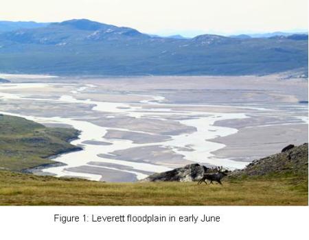
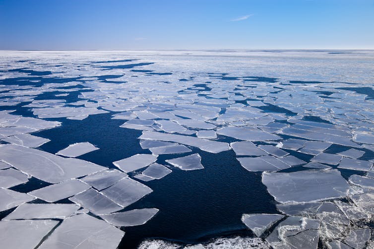
During the course of my stay at the University of Bristol-led field site near Leverett glacier in south-west Greenland, I witnessed the start of what has since been identified as one of the most significant Greenland melt years over the past century. Over that time Leverett glacier’s subglacial drainage river, fed by the melting ice sheet surface together with stored meltwater from the bed, had altered from a small stream to a raging torrent. Although this is usual for a glacial river during a melt season in Greenland, the scale of change was unprecedented. Temperatures around camp far exceeded my expectations. I packed expedition gear expecting Arctic summer temperatures of around 10°C – a little higher than I had previously experienced in the northerly island archipelago of Svalbard. What I experienced were temperatures sometimes reaching 20°C. In our camp mess tent where we cooked and ate our meals the temperature would sometimes exceed 30°C – shorts and t-shirt weather – were it not for the thousands of mosquitoes that were thriving in the warmer weather. In June I often found myself processing samples in the science tent with beads of sweat on my brow.

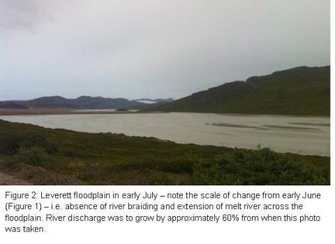
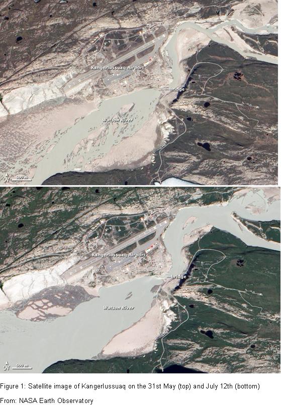
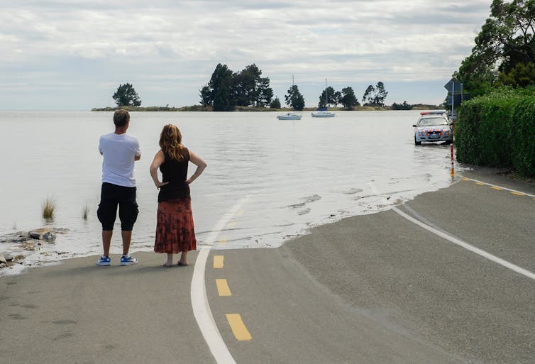
When the discharge of the river exiting the margin of Leverett glacier hit around 500 m3/s in late June (over six times that of the average River Thames discharge when flowing through London), it was evident to all of the camp that the 2012 melt season was going to be much larger than in previous years. Over the period that Leverett catchment has been studied (2009-), river discharge usually reaches a high of 405 m3/s, and that was in early August – more than a month after this high (and therefore after a month’s more melt). At that time a bridge crossing the glacial meltwater river in the nearest town, Kangerlussuaq, approximately 25 km downstream (Watson River, fed by Leverett glacier and two other large glaciers in the area), had to be closed as the amount of water deemed it unsafe. I’ve recently been informed that discharge of Leverett river has subsequently hit more than 800 m3/s since I left camp – nearly twice that of the previous high. At the same time Watson River discharge at Kangerlussuaq was nearly double its previous high (3500 m3/s – more than the average discharge of the Nile), and in dramatic fashion has washed away the same bridge that was closed in 2010 (see http://www.guardian.co.uk/environment/picture/2012/jul/27/glaciers-flooding?newsfeed=true# and http://www.guardian.co.uk/environment/2012/jul/25/greenland-glacier-bridge-destroyed-video?newsfeed=true). Although a trend for higher melt season discharge has been observed, locals and scientists in the Kangerlussuaq area have all been taken aback by the magnitude of change experienced this year (http://www.ouramazingplanet.com/3254-greenland-flooding.html).

As this was my first field season in Greenland it was difficult for me to grasp the scale of change from previous years. Ben Linhoff, an isoptope geochemist from Woods Hole Oceanographic Institute in Massachusetts, USA, has been in camp during the 2011 and 2012 melt seasons, and was surprised by the difference in temperature and river size between the two years. He has documented the scale of change on his Scientific American blog (http://blogs.scientificamerican.com/expeditions/tag/following-the-ice/), and in a short video with Andrew Tedstone of the University of Edinburgh (http://www.whoi.edu/page.do?pid=80757&cl=82073&tid=5122). Ben comments that air temperatures in camp are substantially warmer than in 2011 and that glacial moraine deposited by Leverett glacial hundreds of years ago (possibly during the Little Ice Age) was being eroded by Leverett river – likely for the first time in decades. Dave Chandler, a University of Bristol researcher, camped within the ice sheet interior, 40km from the margin, has also been surprised by the warm temperatures. During the 2011 melt season he found that the temperature on the ice very rarely exceeded freezing at night. In contrast, the temperature has stayed above freezing throughout most of June and July at a similar point on the ice this year. Higher temperatures and the lack of freezing conditions on the ice sheet interior mean that more glacial ice has melted on the surface. This water is then thought to be routed to the bed through conduits know as moulins. At the bed the meltwater joins a large subglacial channel that flows under the ice and exits the glacier via a portal such as that which exists on Leverett glacier. The discharge of these subglacial rivers is thus indicative of the amount of ice melt.