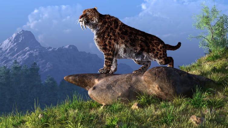
ManuMata / shutterstock
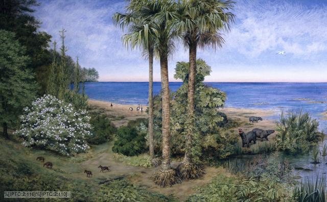
Around 252 million years ago, the world suddenly heated up. Over a geologically brief period of tens of thousands of years, 90% of species were wiped out. Even insects, which are rarely touched by such events, suffered catastrophic losses. The Permian-Triassic mass extinction, as it’s known, was the greatest of the “big five” mass extinctions in Earth’s history.
Scientists have generally blamed the mass extinction on greenhouse gases released from a vast network of volcanoes which covered much of modern day Siberia in lava. But the volcanic explanation was incomplete. In our new study, we show that an enormous El Niño weather pattern in the world’s major ocean added to climate chaos and led to extinctions spreading across the globe.
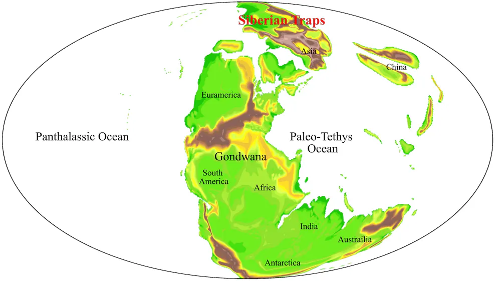
It’s easy to see why volcanoes were blamed. The onset of extinction coincides almost perfectly with the beginning of the second phase of volcanism in the region known as the Siberian Traps. This led to acid rain, oceans losing their oxygen and, most notably, temperatures beyond the tolerance levels of almost all organisms. It was the greatest episode of global warming in the past 500 million years.
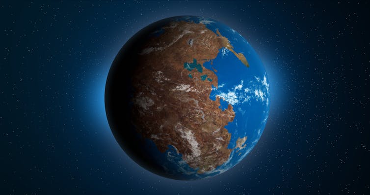
The world 252 million years ago
However, there were outstanding questions for proponents of this seemingly simple extinction scenario: when the tropics became too hot, why did species not just migrate to cooler, higher latitudes (as is happening today)? If warming was sudden and rapid, why did species on land die off tens of thousands of years before those in the sea?
There have also been many instances of volcanic eruptions of similar scale, and even other episodes of rapid warming, but why did none of these cause a similarly catastrophic mass extinction?
Our new study reveals that the oceans rapidly heated up all across the world’s low and mid latitudes. Normally, it gets cooler as you move away from the tropics, but not this time. It simply became too hot for life in too many places.
A world prone to extremes
Using a state-of-the-art computer program, we were able to simulate what the weather and climate was like 252 million years ago. We found that, even before the rapid warming, the world would have been prone to extremes of temperature and rainfall.
That’s a consequence of all the land at the time forming into one large supercontinent, Pangaea. This meant that the climates we see today at the centre of continents – dry, with hot summers and freezing winters – were magnified.
Pangaea was surrounded by a vast ocean, Panthalassa, the surface of which would fluctuate between warm and cool periods over the years, much like the El Niño phenomenon in the Pacific today. Yet once the mass Siberian volcanism started and carbon dioxide in the atmosphere increased, those prehistoric El Niños became more intense and lasted longer thanks to the larger Panthalassa ocean being able to store more heat.
An El Niño far stronger than anything today

Alex Farnsworth
These El Niños had a profound impact on life on land, and kicked off a sequence of events that made the climate more and more extreme. Temperatures got hotter, especially in the tropics, and huge droughts and fires caused tropical forests to die off.
This in turn was bad news for the climate, as less carbon was stored by trees, allowing more to linger in the atmosphere, leading to further warming, and even stronger and longer El Niños.
252 million years ago, pre crisis:
Alex Farnsworth
These stronger El Niños caused the extreme temperatures and droughts to push outside of the tropics towards the poles, and more vegetation died off and more carbon was released. Over tens of thousands of years, extreme temperatures spread over much of the world’s surface. Eventually, the warming began to harm life in the oceans, particularly tiny organisms at the bottom of the food chain.
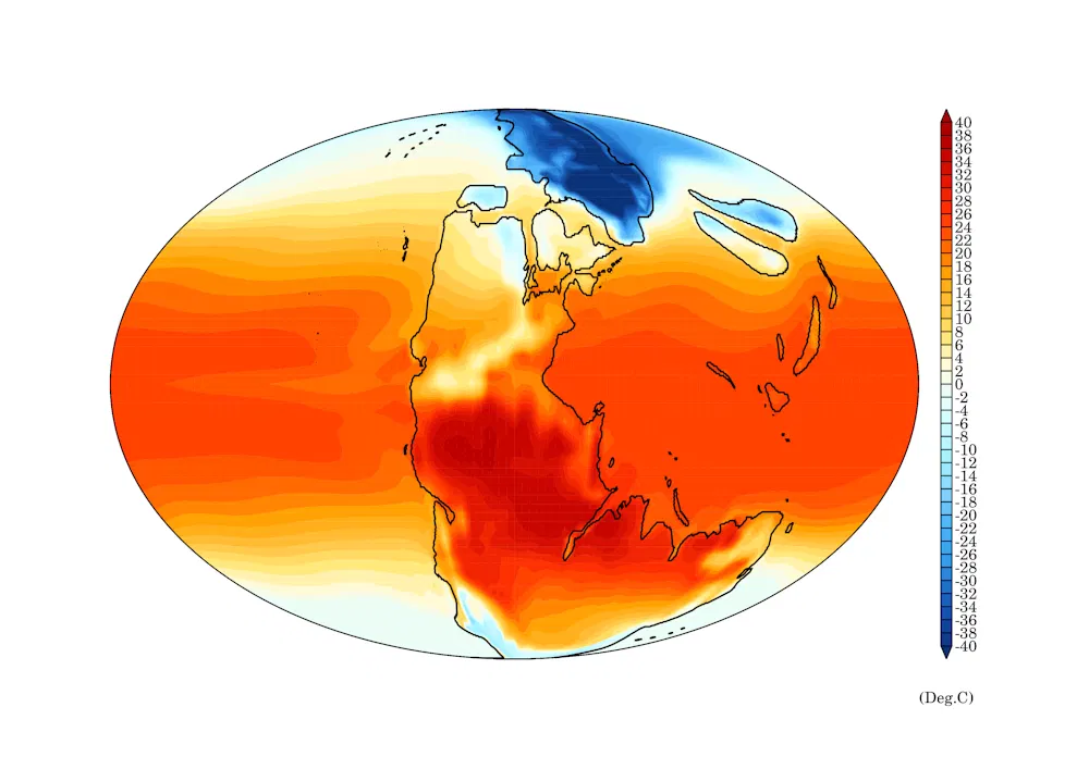
…and at the peak of the extinction:
Alex Farnsworth
During the peak of the crisis, in a world that was already warming thanks to volcanic gases, an El Niño would boost average temperatures by a further 4°C. That’s more than three times the total warming we have caused over the past few centuries. Back then, the El Niño-charged climate would have regularly seen peak daytime temperatures on land of 60°C or more.
The future of El Niño
In recent years El Niños have caused major changes to rainfall and temperature patterns, around the Pacific and even further afield. A strong El Niño was a factor in record-breaking temperatures through 2023 and 2024.
Fortunately, such events typically only last a few years. However, on top of human-caused warming, even these smaller scale El Niños of the present day may be enough to push fragile ecosystems beyond their limit.
El Niño is predicted to become more variable as the climate changes, though we should note that the oceans are still yet to fully respond to current warming rates. At present, nobody is forecasting another mass extinction on the scale of the one 252 million years ago, but that event provides a worrying snapshot of what happens when El Niño gets out of control.![]()
———————————
This blog is written by Dr Alex Farnsworth, Senior Research Associate in Meteorology, University of Bristol; David Bond, Palaeoenvironmental Scientist, University of Hull, and Paul Wignall, Professor of Palaeoenvironments, University of Leeds. This article is republished from The Conversation under a Creative Commons license. Read the original article.