Mock COP26: Convincing, Cooperating and Collaborating


Glasgow COP26 presentation, preliminary discussion, and negotiation rounds 1 & 2

On 11th November at 10am around 60 A-level students from schools across Bristol gathered to participate in this year’s Mock COP26, hosted by Jack Nicholls, Emilia Melville, and Camille Straatman from the Cabot Institute for the Environment. After a resounding success from the first Mock COP, which took place online in March 2021, there was real excitement and anticipation building for the in-person event which would be held in the Great Hall of the Wills Memorial Building.

The morning kicked off with an engaging presentation by Jack, Emilia, and Camille, outlining the objectives of the upcoming COP26 in Glasgow. There had been much discussion surrounding the COP in the public sphere in the prior weeks, so it was interesting to see a summary of where things stand in the time since the Paris Agreement and what the potential outcomes of this COP may be.

The negotiations began with preliminary intra-group discussions, facilitated by a group of 12 postgraduate students. Each group defined their stance on each of the COP resolutions, ranging from option A, the most radical response, to C, the most conservative. It was evident from the off that these students were highly knowledgeable and passionate about the environmental, sociological, and economic impacts of each resolution, and as a result, each group wasted no time in prioritising the resolutions that would benefit their actor the most. Brazil factored in its current economic and development situation, as well as the Amazon’s critical role in the ecosystem balance, choosing to prioritise climate finance, natural protection and conservation and protecting climate refugees. For the International Indigenous Peoples Forum on Climate Change (IIFPCC), giving protected status to 50% of Earth’s natural areas by 2050 was defined as the most important resolution, whereas Shell chose to focus on phasing out coal, with the understanding that this would take the onus off the oil industry. Each group presented their ideal resolutions in a clear and concise manner.

The atmosphere really started to build in the hall when the first round of negotiations began. China faced Greenpeace in a heated discussion on coal usage while the IIFPCC negotiated with the USA on protecting indigenous populations. The United Nations High Commissioner for Refugees found alignment with Brazil on many of the resolutions, namely achieving net-zero emissions by 2050, natural protection and conservation to 30% of Earth’s natural areas and protecting climate refugees. In round two of negotiations, we saw Shell and the International Monetary Fund categorically disagree on the timeline for transition to Zero Emissions Vehicles, eventually compromising on a B resolution to have all new vehicle sales as zero-emission by 2040. Brazil was happy in supporting the IIPFCC in resolution 7a. (All countries must allow people fleeing from natural disasters, environmental degradation, and sea level rise to enter their countries and make their new homes there). Brazil and IIPFCC made an alliance to encourage USA toward resolution 7a, instead of their preferred 7b (Countries at risk of extinction from sea level rise should be provided with new land to settle and move their people to OR be provided with financial help to buy land in other nations). China and the Alliance of Small Island States (AOSIS) clash on coal usage, with AOSIS pushing back with a suggestion of image control, but ultimately China held strong on their decision.

Negotiation rounds 3 & 4, voting, and deputy mayor’s speech

The UK showed their tactical abilities and their knowledge in the negotiations with Greenpeace, but Greenpeace did not cede to their demands and manage to agree to a deal.  The IIPFCC was determined to protect indigenous land and communities, but their quest was heavily challenged by Shell. There was no common ground in the negotiation with this petrol giant, so the IIPFCC had to ensure an allyship with Brazil if they wanted to ensure the protection of the indigenous. On round four, Shell tried to sway some votes from China and Sweden, but while agreements were found with the former, the latter country was not going to let Shell influence their values. The tête-à-tête became lively as neither Shell nor Sweden were willing to compromise, resulting in a rather unsuccessful attempt of finding complicity.

After four intense rounds of negotiating, the voting began. Were all parties going to remain faithful to the agreements established during the negotiations? Or would some throw a curve ball, changing their minds at the last minute? The pondered tactics of the IIPFCC were successful, as they managed to lock Brazil’s and the USA’s support on their most valued resolutions. All parties pondered thoroughly on how to best use their votes, and it seemed that this meant that some agreements had been silently retracted, when some astonished reactions followed the raise of hands here and there.

The conference was finally over and many parties, including Brazil and Greenpeace, could celebrate the victory of the resolutions agreed upon. Yet, it was clear that a bittersweet aftertaste was left in the mouths of some parties, who did not manage to persuade enough. The heated debate had ended, and what was done was done, but one more surprise was awaiting our participants. Deputy Mayor Asher Craig had been sitting on the sidelines for a few instances already, assisting in the final yet most heated rounds of the conference. She was there, observing our pupils in awe as they got into character and avidly fought for their beliefs. The Deputy Mayor was impressed by the passion of these young minds and how much they are invested in the cause; she was proud to see that young generations care about the environment and our planet, as they came up with ideas for change that they would like to see more in the Bristol. The innovativeness and creativity of the students was remarkable in her eyes, as she proceeded to give an inspiring and uplifting speech on the efforts currently being made by the City Council to respond to the climate emergency. The mock COP26 was a more than a successful event, and as everyone waited for the results of the conference in Glasgow, we all wished that our simulation had been real.

Watch the students in action in this short video created by Particle Productions and funded by Bristol City Council.

————————————–

This blog is written by Sonia Pighini and Jennifer Malone, who are students on the Cabot Institute for the Environment Master’s by Research.

Jennifer Malone
Currently studying for a Master’s by Research in Global  Environmental Challenges from the Cabot Institute for the Environment, Jennifer’s research is centred on food system decarbonisation within the scope of UK food policy and community practice.
Sonia Pigini

Sonia is an international student in the MscR programme Global Environmental Challenges. Their research focuses on people-centred sustainable food system transitions in Bristol. They are particularly interested in exploring the potential for a more decentralised food system in the city, which empowers local producers, engages consumers and that keeps aspects such as justice and inclusion at its heart.

Image credit (image at top of blog): Jack Pitts

Humanity is compressing millions of years of natural change into just a few centuries

The near future may be similar to the mid-Pliocene warm period a few million years ago.
Daniel Eskridge / shutterstock

Many numbers are swirling around the climate negotiations at the UN climate summit in Glasgow, COP26. These include global warming targets of 1.5℃ and 2.0℃, recent warming of 1.1℃, remaining CO₂ budget of 400 billion tonnes, or current atmospheric CO₂ of 415 parts per million.

It’s often hard to grasp the significance of these numbers. But the study of ancient climates can give us an appreciation of their scale compared to what has occurred naturally in the past. Our knowledge of ancient climate change also allows scientists to calibrate their models and therefore improve predictions of what the future may hold.

Recent climate changes in context.
IPCC AR6, chapter 2

Recent work, summarised in the latest report of the Intergovernmental Panel on Climate Change (IPCC), has allowed scientists to refine their understanding and measurement of past climate changes. These changes are recorded in rocky outcrops, sediments from the ocean floor and lakes, in polar ice sheets, and in other shorter-term archives such as tree rings and corals. As scientists discover more of these archives and get better at using them, we have become increasingly able to compare recent and future climate change with what has happened in the past, and to provide important context to the numbers involved in climate negotiations.

For instance one headline finding in the IPCC report was that global temperature (currently 1.1℃ above a pre-industrial baseline) is higher than at any time in at least the past 120,000 or so years. That’s because the last warm period between ice ages peaked about 125,000 years ago – in contrast to today, warmth at that time was driven not by CO₂, but by changes in Earth’s orbit and spin axis. Another finding regards the rate of current warming, which is faster than at any time in the past 2,000 years – and probably much longer.

But it is not only past temperature that can be reconstructed from the geological record. For instance, tiny gas bubbles trapped in Antarctic ice can record atmospheric CO₂ concentrations back to 800,000 years ago. Beyond that, scientists can turn to microscopic fossils preserved in seabed sediments. These properties (such as the types of elements that make up the fossil shells) are related to how much CO₂ was in the ocean when the fossilised organisms were alive, which itself is related to how much was in the atmosphere. As we get better at using these “proxies” for atmospheric CO₂, recent work has shown that the current atmospheric CO₂ concentration of around 415 parts per million (compared to 280 ppm prior to industrialisation in the early 1800s), is greater than at any time in at least the past 2 million years.

chart showing climate changes over history
An IPCC graphic showing climate changes at various points since 56 million years ago. Note most rows show changes over thousands or millions of years, while the top row (recent changes) is just a few decades.
IPCC AR6, chapter 2 (modified by Darrell Kaufman)

Other climate variables can also be compared to past changes. These include the greenhouse gases methane and nitrous oxide (now greater than at any time in at least 800,000 years), late summer Arctic sea ice area (smaller than at any time in at least the past 1,000 years), glacier retreat (unprecedented in at least 2,000 years) sea level (rising faster than at any point in at least 3,000 years), and ocean acidity (unusually acidic compared to the past 2 million years).

In addition, changes predicted by climate models can be compared to the past. For instance an “intermediate” amount of emissions will likely lead to global warming of between 2.3°C and 4.6°C by the year 2300, which is similar to the mid-Pliocene warm period of about 3.2 million years ago. Extremely high emissions would lead to warming of somewhere between 6.6°C and 14.1°C, which just overlaps with the warmest period since the demise of the dinosaurs – the “Paleocene-Eocene Thermal Maximum” kicked off by massive volcanic eruptions about 55 million years ago. As such, humanity is currently on the path to compressing millions of years of temperature change into just a couple of centuries.

Small animals in a forest
Many mammals, like these horse-ancestors ‘Eohippus’, first appeared after a sudden warm period 55 million years ago.
Daniel Eskridge / shutterstock

Distant past can held predict the near future

For the first time in an IPCC report, the latest report uses ancient time periods to refine projections of climate change. In previous IPCC reports, future projections have been produced simply by averaging results from all climate models, and using their spread as a measure of uncertainty. But for this new report, temperature and rainfall and sea level projections relied more heavily on those models that did the best job of simulating known climate changes.

Part of this process was based on each individual model’s “climate sensitivity” – the amount it warms when atmospheric CO₂ is doubled. The “correct” value (and uncertainty range) of sensitivity is known from a number of different lines of evidence, one of which comes from certain times in the ancient past when global temperature changes were driven by natural changes in CO₂, caused for example by volcanic eruptions or change in the amount of carbon removed from the atmosphere as rocks are eroded away. Combining estimates of ancient CO₂ and temperature therefore allows scientists to estimate the “correct” value of climate sensitivity, and so refine their future projections by relying more heavily on those models with more accurate climate sensitivities.

Overall, past climates show us that recent changes across all aspects of the Earth system are unprecedented in at least thousands of years. Unless emissions are reduced rapidly and dramatically, global warming will reach a level that has not been seen for millions of years. Let’s hope those attending COP26 are listening to messages from the past.

——————————

This blog is written by Cabot Institute for the Environment member Dan Lunt, Professor of Climate Science, University of Bristol and Darrell Kaufman, Professor of Earth and Environmental Sciences, Northern Arizona University

This article is republished from The Conversation under a Creative Commons license. Read the original article.

Dan Lunt


Read all blogs in our COP26 blog series:

Five satellite images that show how fast our planet is changing


Stocktrek Images, Inc. / Alamy

You have probably seen satellite images of the planet through applications like Google Earth. These provide a fascinating view of the surface of the planet from a unique vantage point and can be both beautiful to look at and useful aids for planning. But satellite observations can provide far more insights than that. In fact, they are essential for understanding how our planet is changing and responding to global heating and can do so much more than just “taking pictures”.

It really is rocket science and the kind of information we can now obtain from what are called Earth observation satellites is revolutionising our ability to carry out a comprehensive and timely health check on the planetary systems we rely on for our survival. We can measure changes in sea level down to a single millimetre, changes in how much water is stored in underground rocks, the temperature of the land and ocean and the spread of atmospheric pollutants and greenhouse gases, all from space.

Here I have selected five striking images that illustrate how Earth observation data is informing climate scientists about the changing characteristics of the planet we call home.

1. The sea level is rising – but where?

Map showing global sea level rise
The sea is rising quickly – but not evenly.
ESA/CLS/LEGOS, CC BY-SA

Sea level rise is predicted to be one of the most serious consequences of global heating: under the more extreme “business-as-usual” scenario, a two-metre rise would flood 600 million people by the end of this century. The pattern of sea surface height change, however, is not uniform across the oceans.

This image shows mean sea level trends over 13 years in which the global average rise was about 3.2mm a year. But the rate was three or four times faster in some places, like the south western Pacific to the east of Indonesia and New Zealand, where there are numerous small islands and atolls that are already very vulnerable to sea level rise. Meanwhile in other parts of the ocean the sea level has barely changed, such as in the Pacific to the west of North America.

2. Permafrost is thawing

Source: ESA

Permafrost is permanently frozen ground and the vast majority of it lies in the Arctic. It stores huge quantities of carbon but when it thaws, that carbon is released as CO₂ and an even more potent greenhouse gas: methane. Permafrost stores about 1,500 billion tonnes of carbon – twice as much as in the whole of the atmosphere – and it is incredibly important that carbon stays in the ground.

This animation combines satellite, ground-based measurements of soil temperature and computer modelling to map the permafrost temperature at depth across the Arctic and how it is changing with time, giving an indication of where it is thawing.

3. Lockdown cleans Europe’s skies

Source: ESA

Nitrogen dioxide is an atmospheric pollutant that can have serious health impacts, especially for those who are asthmatic or have weakened lung function, and it can increase the acidity of rainfall with damaging effects on sensitive ecosystems and plant health. A major source is from internal combustion engines found in cars and other vehicles.

This animation shows the difference in NO₂ concentrations over Europe before national pandemic-related lockdowns began in March 2020 and just after. The latter shows a dramatic reduction in concentration over major conurbations such as Madrid, Milan and Paris.

4. Deforestation in the Amazon

Credits: ESA/USGS/Deimos Imaging

Tropical forests have been described as the lungs of the planet, breathing in CO₂ and storing it in woody biomass while exhaling oxygen. Deforestation in Amazonia has been in the news recently because of deregulation and increased forest clearing in Brazil but it had been taking place, perhaps not so rapidly, for decades. This animation shows dramatic loss of rainforest in the western Brazilian state of Rondonia between 1986 and 2010, as observed by satellites.

5. A megacity-sized iceberg

Source: ESA

The Antarctic Ice Sheet contains enough frozen water to raise global sea level by 58 metres if it all ended up in the ocean. The floating ice shelves that fringe the continent act as a buffer and barrier between the warm ocean and inland ice but they are vulnerable to both oceanic and atmospheric warming.

This animation shows the break-off of a huge iceberg dubbed A-74, captured by satellite radar images that have the advantage they can “see” through clouds and operate day or night and are thus unaffected by the 24 hours of darkness that occurs during the Antarctic winter. The iceberg that forms is 1,270 km² in area which is about the same size as Greater London.

These examples illustrate just a few ways in which satellite data are providing unique, global observations of key components of the climate system and biosphere that are essential for our understanding of how the planet is changing. We can use this data to monitor those changes and improve models used to predict future change. In the run up to the vitally important UN climate conference, COP26 in Glasgow this November, colleagues and I have produced a briefing paper to highlight the role Earth observation satellites will play in safeguarding the climate and other systems that we rely on to make this beautiful, fragile planet habitable.The Conversation

————————–

This blog is written by Cabot Institute for the Environment member Jonathan Bamber, Professor of Physical Geography, University of Bristol.

This article is republished from The Conversation under a Creative Commons license. Read the original article.

Jonathan Bamber

Frozen in time: reflections on a PhD and the history of Antarctica

In March 2020, the third and final instalment of my PhD research made its way into Climate of the Past. In that article, I do my best to synthesise all I learnt over 5 years about an event that occurred 34 million years ago called the Eocene-Oligocene Transition. (Just so we are all on the same page: palaeoclimate scientists are interested in this period of the Earth’s history as it is when the first major Antarctic Ice Sheet appeared; before then Antarctica was warm and at least partially forested.)

An image of what Antarctica might have looked like at the onset of the Eocene-Oligocene Transition.

Four and a half years ago I wrote a piece for the Cabot Institute Blog about using a climate model to understand this point in the Earth’s history, and how many questions remained in our understanding. Why was the Earth so hot beforehand? What caused it to cool and eventually for Antarctica to glaciate? What other important changes would have occurred around the world at this time? At the time, I focussed particularly on the latter question.

The more time I spent trying to answer some of these questions, predictably (as is the way with science), the more complex some of them became. In the end, for my own peace of mind, I simply tried to bring together as much information as I could from lots of different sources to try to create a picture with some sort of clarity. I focussed on the high latitude Southern Hemisphere, because that is where a lot of the action was occurring at the Eocene-Oligocene Transition and it is also where models potentially have some difficulties in reproducing the climate.

To build up this picture, I used multiple climate model simulations of the period from two different modelling groups and compared these to the biggest dataset of proxy records of Southern Hemisphere climate 34 million years ago that I could compile by myself. Just reading and compiling all of the data from papers took me around a year. Not solidly (I had lots of other things to do too), but even still, reading papers solidly is very difficult in my opinion. Synthesising all of that different information into something coherent in my head is also something that I cannot force to happen quickly. It comes when it is ready.

Some of the complied proxy data for the high latitude Southern Hemisphere the Eocene-Oligocene Transition included in Kennedy-Asser et al. (2020).
In the end for this paper, I generated no primary data myself. It is all secondary data, either provided by other researchers I work with or taken from this very slow and lengthy review of scientific literature. Maybe, back at the start, that is not how I had pictured the finale of my thesis might look. Maybe the plan was to build up to some exceptional new result that I discovered, with data I produced with my own hands. But that wasn’t the case and, to be honest, I think it is better the way it is. Science is, and should be, a collaborative effort. In the spirit of this, I put all of the data I compiled and used, including all of my analysis scripts and detailed notes of where I obtained secondary data, up on the Open Science Framework. This way I hope the science can keep collaborating and continue growing.
Two thirds of my thesis were based on ‘my own’ data, messing around with a climate model, trying out new ideas, seeing if anything revolutionary popped out. This was really important too: for me to grow as a researcher, to learn about how the model works and to try to generate some outside-the-box ideas. Occasionally, of course, something truly revolutionary will be discovered. In the end, however, my conclusion is that model results often lack meaning by themselves: they need observations or proxy records to go with them to provide some sort of truth of what really happened, whether that is outside right now or 34 million years ago.
My new paper finds very similar things about why the Earth changed so much at the Eocene-Oligocene Transition to earlier research carried out nearly 20 years ago. It doesn’t challenge or rewrite everything we know, but that’s okay. The main scientific conclusion from my paper is that incorporating all of this data is actually essential to coming to the same conclusion as the research from many years ago. Without the inclusion of the boring, extensive data review, I might have quickly, excitedly jumped to a different conclusion that, on balance, seems less likely to be correct.
Much like this paper brings together different existing scientific data to compliment research built up over many years, it also brings together my own work and thoughts. It took many years, but it wouldn’t make sense to rush it: the conclusions take a bit of time, even if all of the data and answers are already out there.
————————————

This blog is written by Cabot Institute member Alan Kennedy-Asser, a Research Associate at the School of Geographical Sciences, University of Bristol. You can follow Alan on Twitter @EzekielBoom.

Alan Kennedy-Asser


Learning about cascading hazards at the iRALL School in China

Earlier this year, I wrote about my experiences of attending an interdisciplinary workshop in Mexico, and how these approaches foster a rounded approach to addressing the challenges in communicating risk in earth sciences research. In the field of geohazards, this approach is increasingly becoming adopted due to the concept of “cascading hazards”, or in other words, recognising that when a natural hazard causes a human disaster it often does so as part of a chain of events, rather than as a standalone incident. This is especially true in my field of research; landslides. Landslides are, after all, geological phenomena studied by a wide range of “geoscientists” (read: geologists, geomorphologists, remote sensors, geophysicists, meteorologists, environmental scientists, risk assessors, geotechnical and civil engineers, disaster risk-reduction agencies, the list goes on). Sadly, these natural hazards affect many people across the globe, and we have had several shocking reminders in recent months of how landslides are an inextricable hazard in areas prone to earthquakes and extremes of precipitation.

The iRALL, or the ‘International Research Association on Large Landslides’, is a consortium of researchers from across the world trying to adopt this approach to understanding cascading hazards, with a particular focus on landslides. I was lucky enough to attend the ‘iRALL School 2018: Field data collection, monitoring and modelling of large landslides’ in October this year, hosted by the State Key Laboratory of Geohazard Prevention and Geoenvironment Protection (SKLGP) at Chengdu University of Technology (CDUT), Chengdu, China. The school was attended by over 30 postgraduate and postdoctoral researchers working in fields related to landslide and earthquake research. The diversity of students, both in terms of subjects and origins, was staggering: geotechnical and civil engineers from the UK, landslide specialists from China, soil scientists from Japan, geologists from the Himalaya region, remote sensing researchers from Italy, earthquake engineers from South America, geophysicists from Belgium; and that’s just some of the students! In the two weeks we spent in China, we received presentations from a plethora of global experts, delivering lectures in all aspects of landslide studies, including landslide failure mechanisms, hydrology, geophysics, modelling, earthquake responses, remote sensing, and runout analysis amongst others. Having such a well-structured program of distilled knowledge delivered by these world-class researchers would have been enough, but one of the highlights of the school was the fieldwork attached to the lectures.

The scale of landslides affecting Beichuan County is difficult to grasp: in this photo of the Tangjiwan landslide, the red arrow points to a one story building. This landslide was triggered by the 2008 Wenchuan earthquake, and reactivated by heavy rainfall in 2016.

The first four days of the school were spent at SKLGP at CDUT, learning about the cascading hazard chain caused by the 2008 Wenchuan earthquake, another poignant event which demonstrates the interconnectivity of natural hazards. On 12th May 2008, a magnitude 7.9 earthquake occurred in Beichuan County, China’s largest seismic event for over 50 years. The earthquake triggered the immediate destabilisation of more than 60,000 landslides, and affected an area of over 35,000 km2; the largest of these, the Daguangbao landslide, had an estimated volume of 1.2 billion m3 (Huang and Fan, 2013). It is difficult to comprehend numbers on these scales, but here’s an attempt: 35,000 km2 is an area bigger than the Netherlands, and 1.2 billion m3 is the amount of material you would need to fill the O2 Arena in London 430 times over. These comparisons still don’t manage to convey the scale of the devastation of the 2008 Wenchuan earthquake, and so after the first four days in Chengdu, it was time to move three hours north to Beichuan County, to see first-hand the impacts of the earthquake from a decade ago. We would spend the next ten days here, continuing a series of excellent lectures punctuated with visits to the field to see and study the landscape features that we were learning about in the classroom.

The most sobering memorial of the 2008 Wenchuan earthquake is the ‘Beichuan Earthquake Historic Site’, comprising the stabilised remains of collapsed and partially-collapsed buildings of the town of Old Beichuan. This town was situated close to the epicentre of the Wenchuan earthquake, and consequently suffered huge damage during the shaking, as well as being impacted by two large landslides which buried buildings in the town; one of these landslides buried a school with over 600 students and teachers inside. Today, a single basketball hoop in the corner of a buried playground is all that identifies it as once being a school. In total, around 20,000 people died in a town with a population of 30,000. Earth science is an applied field of study, and as such, researchers are often more aware of the impact of their research on the public than in some other areas of science. Despite this, we don’t always come this close to the devastation that justifies the importance of our research in the first place.

River erosion damaging check-dams designed to stop debris flows is still a problem in Beichuan County, a decade after the 2008 Wenchuan earthquake.

It may be a cliché, but seeing is believing, and the iRALL School provided many opportunities to see the lasting impacts of large slope failures, both to society and the landscape. The risk of debris flows resulting from the blocking of rivers by landslides (a further step in the cascading hazard chain surrounding earthquakes and landslides) continues to be a hazard threatening people in Beichuan County today. Debris flow check-dams installed after the 2008 Wenchuan earthquake are still being constantly maintained or replaced to provide protection to vulnerable river valleys, and the risk of reactivation of landslides in a seismically active area is always present. But this is why organisations such as the iRALL, and their activities such as the iRALL School are so important; it is near impossible to gain a true understanding of the impact of cascading hazards without bringing the classroom and the field together. The same is true when trying to work on solutions to lessen the impact of these cascading hazard chains. It is only by collaborating with people from a broad range of backgrounds, skills and experiences can we expect to come up with effective solutions that are more than the sum of their parts.

—————
This blog has been reposted with kind permission from James Whiteley.  View the original blog on BGS Geoblogy.   This blog was written by James Whiteley, a geophysicist and geologist at University of Bristol, hosted by British Geological Survey. Jim is funded through the BGS University Funding Initiative (BUFI). The aim of BUFI is to encourage and fund science at the PhD level. At present there are around 130 PhD students who are based at about 35 UK universities and research institutes. BUFI do not fund applications from individuals.

Back to the Future ‘Hothouse’

Our current global warming target and the trajectory it places us on, towards a future ‘Hothouse Earth’, has been the subject of much recent discussion, stimulated by a paper by Will Steffen and colleagues.  In many respects, the key contribution of this paper and similar work is to extend the temporal framing of our climate discussions, beyond 2100 for several centuries or more.  Analogously, it is useful to extend our perspective backwards to similar time periods, to reflect on the last time Earth experienced such a Hothouse state and what it means.

The Steffen et al paper allows for a variety of framings, all related to the range of natural physical, biological and chemical feedbacks that will amplify or mitigate the human intervention in climate.  [Note: the authors frame their paper around the concept of a limited number of steady state scenarios/temperatures for the Earth.  They then argue that aiming for 2C, potentially an unstable state, could trigger feedbacks tipping the world towards the 4C warmer Hothouse.  I find that to be somewhat simplistic given the diversity of climate states that have existed, if even transiently, over the past 15 million years, but that is a discussion for another day.] From my perspective, the most useful framing – and one that remains true to the spirit of the paper is this: We have set a global warming limit of 2C by 2100, with an associated carbon budget. What feedback processes will that carbon budget and warming actually unleash over the coming century,  how much additional warming will they add, and when?

That is a challenging set of questions that comes with a host of caveats, most related to the profound uncertainty in the interlinked biogeochemical processes that underpin climate feedbacks. For example, as global warming thaws the permafrost, will it release methane (with a high global warming potential than carbon dioxide)? Will the thawed organic matter oxidise to carbon dioxide or will it be washed and buried in the ocean? And will the increased growth of plants under warmer conditions lead instead to the sequestration of carbon dioxide? The authors refer to previous studies that suggest a permafrost feedback yielding an additional 0.1C warming by the end of the century; but there is great uncertainty in both the magnitude of that impact and its timing.

And timing is the great question at the heart of this perspective piece.  I welcome it, because too often our perspective is fixed on the arbitrary date of 2100, knowing full well that the Earth will continue to warm and ice continue to melt long after that date.  In this sense, Steffen et al is not a contradiction to what has been reported from the IPCC but an expansion on it.

Classically, we discuss these issues in terms of fast and slow feedbacks, but in fact there is a continuum between near instantaneous feedbacks and those that act over hundreds, thousands or even millions of years.  A warmer atmosphere will almost immediately hold more water vapour, providing a rapid positive feedback on warming – and one that is included in all of those IPCC projections.  More slowly, soil carbon, including permafrost, will begin to oxidise, with microbial activity stimulated and accelerated under warmer conditions – a feedback that is only just now being included in Earth system models.  And longer term, all manner of processes will come into play – and eventually, they will include the negative feedbacks that have helped regulate Earth’s climate for the past 4 billion years.

There is enough uncertainty in these processes to express caution in some of the press’s more exuberant reporting of this topic.  But lessons from the past certainly underscore the concerns articulated by Steffen et al.  We think that the last time Earth had 410 ppm CO2, a level similar to what you are breathing right now, was the Pliocene about 3 million years ago.  This was a world that was 1 to 2C warmer than today (i.e. 2 to 3C warmer than the pre-industrial Earth) and with sea levels about 10 m higher.  This suggests that we are already locked into a world that far exceeds the ambitions and targets of the Paris Agreement.  This is not certain as we live on a different planet and one where the great ice sheets of Greenland and Antarctica might not only be victims of climate change but climate stabilisers through ice-sheet hysteresis. And even if a Pliocene future is fixed, it might take centuries for that warming and sea level change to be realised.

But that analogue does suggest caution, as advocated by the Hothouse Earth authors.

It also prompts us to ask what the Earth was like the last time its atmosphere held about 500 ppm CO2, similar to the level needed to achieve the Paris Agreement to limit end-of-century warming below 2C.  A useful analogue for those greenhouse gas levels is the Middle Miocene Climate Optimum, which occurred from 17 to 14.7 million years ago.

Figure showing changes in ocean temperature (based on oxygen isotopic compositions of benthic foraminifera) and pCO2 over the past 60 million years (from Palaeo-CO2).  Solid symbols are from the d11B isotope proxy and muted symbols are from the alkenone-based algal carbon isotope fractional proxy. Note the spike in pCO2 associated with the MMCO at about 15 million years ago.

As one would expect for a world with markedly higher carbon dioxide levels, the Miocene was hotter than the climate of today.  And consistent with many of Steffen et al.’s arguments, it was about 4C hotter rather than a mere 2C, likely due to the range of carbon cycle and ice-albedo feedbacks they describe.  But such warmth was not uniform – globally warmer temperatures of 4C manifest as far hotter temperatures in some parts of the world and only slightly warmer temperatures elsewhere. Pollen and microbial molecular fossils from the North Sea, for example, indicate that Northern Europe experienced sub-tropical climates.

But what were the impacts of this warmth?  What is a 4C warmer world like?  To understand that, we also need to understand the other ways in which the Miocene world differed from ours, not just due to carbon dioxide concentrations but also the ongoing movement of the continents and the continuing evolution of life.  In both respects, the Miocene was broadly similar to today.  The continents were in similar positions, and the geography of the Miocene is one we would recognise. But there were subtle differences, including the ongoing uplift of the Himalayas and the yet-to-be-closed gateway between North and South America, and these subtle differences could have had major impacts on Asian climate and the North Atlantic circulation, respectively.

Similarly, the major animal groups had evolved by this point, and mammals had firmly established their dominance in a world separated by 50 million years from the dinosaurs.  Remnant groups from earlier times (hell pigs!) still terrorised the landscape, but many of the groups were the same or closely related to those we would recognise today.  And although hominins would not appear until the end of the Miocene, the apes had become well established, represented by as many as a 100 species. In the oceans, the differences were perhaps more apparent, the seas thriving with the greatest diversity of cetaceans in the history of our planet and associated with them the gigantic macro-predators such as Charcharadon megalodon (The MegTM).

Smithsonian mural showing Miocene Fauna and landscape.

But it is the plants that exhibit the most pronounced differences between modern and Miocene life. Grasses had only recent proliferated across the planet at the time of the MMCO, and the C4 plants had yet to expand to their current dominance. And in this regard, the long-term evolution of Earth’s climate likely played a crucial role.  There are about 8100 species of C4 plants (although this comprises only 3% of the plant species known to us) and most of these are grasses with other notable species being maize and sugar cane. They are distinguished from the dominant C3 plants, which comprise almost all other species, by virtue of their carbon dioxide assimilation biochemistry (the Hatch-Slack mechanism) and their leaf cellular physiology (the Kranz leaf anatomy).  It is a collective package that is exceptionally well adapted to low carbon dioxide conditions, and their global expansion about 7 million years ago was almost certainly related to the long-term decline in carbon dioxide from the high levels of the Middle Miocene. Although C4 plants only represent a small proportion of modern plant species, the Miocene world, bereft of them, would have looked far different than today – lacking nearly half of our modern grass species and by extension clear analogues to the vast African savannahs.

Aside from these, the most profound differences between the Miocene world and that of today would have been the direct impacts of higher global temperatures.  There is strong evidence that the Greenland ice sheet was far reduced in size compared to that of today, and its extent and even whether or not it was a persistent ice sheet or an ephemeral one remains the subject of debate. Similarly, West Antarctica was likely devoid of permanent ice, and the East Antarctic Ice Sheet was probably smaller – perhaps far smaller – than it is today.  And collectively, these smaller ice sheets were associated with a sea level that was about 40 m higher than that of today.

The hot Miocene world would have been different in other ways, including the hydrological cycle.  Although less studied than for other ancient intervals, it is almost certain that elevated warmth – and markedly smaller equator-to-pole temperature differences – would have impacted the global distribution of water.  More water was evidently exported to the high latitudes, resulting in a warmer and vegetated Antarctica where the ice had retreated. It was also likely associated with far more extreme rainfall events, with the hot air able to hold greater quantities of water.  More work is needed, but it is tempting to imagine the impact of these hot temperatures and extreme rainfall events.  They would have eroded the soil and flushed nutrients to the sea, perhaps bringing about the spread of anoxic dead zones, similar to the Oceanic Anoxic Events of the Mesozoic or the dead zones of modern oceans caused by agricultural run-off. Indeed, the Miocene is characterised by the deposition of some very organic-rich rocks, including the North Pacific Monterey Formation, speaking to the occurrence of reduced oxygen levels in parts of these ancient oceans.

****************************************************

It is unclear if our ambitions to limit global warming to 2C by the end of this century really have put us on a trajectory for 4C. It is unclear if we are destined to return to the Miocene.

But if so, the Miocene world is one both similar to but markedly distinct from our own – a world of hotter temperatures, extremes of climate, fewer grasslands, Antarctic vegetation, Arctic forests and far higher sea levels. Crucially, it is not the world for which our current society, its roads, cities, power plants, dams, borders, farmlands and treaties, has been designed.

Moreover, the MMCO Earth is a world that slowly evolved from an even warmer one over millions of years*; and that then evolved over further millions of years to the one in which we now inhabit. It is not a world that formed in a hundred or even a thousand years.  And that leaves us three final lessons from the past.  First, we do not know how the life of this planet, from coral reefs to the great savannahs, will respond to such geologically rapid change.  Second, we do not know how we will respond to such rapid change; if we must adapt, we must learn how to do so creatively, flexibly and equitably.  And third, it is probably not too late to prevent such a future from materialising, but even if it is, we still must act to slow down that rate of change to which we must adapt.

And we still must act to ensure that our future world is only 4C hotter and analogous to the Miocene; if we fail to act, the world will be even hotter, and we will have to extend our geological search 10s of millions of years further into the past, back to the Eocene, to find an even hotter and extreme analogue for our future Hothouse World.

*The final jump into the MMCO appears to have been somewhat more sudden, but still spanned around two-hundred thousand years.  A fast event geologically but not on the timescales of human history.

——————————-
This blog is written by Cabot Institute member Professor Rich Pancost, Head of Earth Sciences at the University of Bristol. This blog has been reposted with kind permission from Rich’s original blog.

Rich Pancost

Sweet love for planet Earth: An ode to bias and fallacy

1. Apocalypse, Albert Goodwin (1903.) At the culmination of 800 paintings, Apocalypse, was the first of Goodwin’s works in which he introduced experimental techniques that marked a distinct departure from the imitations of Turner found in most of his earlier works. [picture courtesy of the Tate online collection.]
Ask for what end the heav’nly bodies shine, 
Earth for whose use? Pride answers, “Tis for mine: 
For me kind Nature wakes her genial pow’r, 
Suckles each herb, and spreads out ev’ry flow’r; 
Annual for me, the grape, the rose renew 
The juice nectareous, and the balmy dew; 
For me, the mine a thousand treasures brings; 
For me, health gushes from a thousand springs; 
Seas roll to waft me, suns to light me rise; 
My foot-stool earth, my canopy the skies.” ’
2. A section of the fifth (V) verse in the first epistle of Alexander Pope’s unfinished Essay on Man, (1733-34.)

Alexander Pope, 18th Century moral poet, pioneer in the use of the heroic couplet, second most quoted writer in the Oxford dictionary of quotations behind Shakespeare and shameless copycat. Coleridge suggested this is what held Pope back from true mastery, but It is beyond question that the results of this imitation cultured some of the finest poetry of the era. Yet still, Pope, the bel esprit of the literary decadence that proliferated within 18th Century written prose and inspiration for the excellence of Byron, Tennyson and Blake, to name but a few; spent a large amount of his creative life imitating the style of Dryden, Chaucer, and John Wilmot, Earl of Rochester. The notion that Pope (2), and Albert Goodwin (1), such precocious and natural talents, would invest so much time in mastering the artistic style of others is curious indeed, it too, provides a broad entry-point for a discussion on the roles of imitation, mimicry and mimesis in human growth, social and societal development.

You live & you learn

Having now formulated a suitable appeal to emotion, which very narrowly avoids the bandwagon, it is worth noting that imitation, and it’s cousins repetition and practice too, represent the way in which an infant might copy its parent’s behaviour, how a young artist may seek a suitably influential model as a teacher or a musician may seek to imitate sounds and transpose these as a compliment to their own polyphony, are a fundamental component in epistemology; the building of knowledge. This understanding has become increasingly important for my own research, whereby repetition and practice have not only become a primary process in developing my own knowledge but have also been important methodological heuristics for establishing imitation and mimicry as primary, collective responses for human survival during exigent situations.

These responses and the systems within which they exist are inherently complex. In developing a robust framework to analyse and evaluate them in relation to flood scenarios for my research (3 and 4) I have utilised the agent-based model to emulate the human response to hydrodynamic data. If you have ever dealt with a HR department, any form of customer service, submitted an academic paper for publishing or bore witness to the wonders of automated passport control then you will be privy to the sentiments of human complexity, as well as our growing dependence on automation to guide us through the orbiting complexity of general life. Raillery aside, these specific examples are rather attenuated situations on which to base broad assessments of human behaviour. The agent-based model itself, a chimera rooted in computational science, born from the slightly sinister cold-war (1953-62) era overlap between computer science, biology and physics and so by implication possessing the ability to model many facets of these disciplines, their related sub-disciplines and inter-disciplines; can provide a panoptic of the broader complexities of human systems and develop our understanding of them.

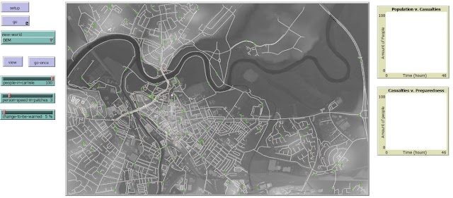
3 (above) & 4 (below). Examples of the agent-based model designed for my own research. The scenario shown is for human response to flooding in Carlisle. The population at risk (green ‘agents’) go about their daily routine until impact from the flood becomes apparent, at which point individuals can choose to go into evacuation mode (red ‘agents’.)

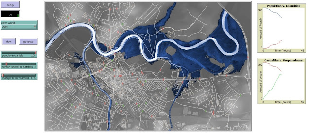
Academically, you may suggest that “these are bold claims!” (others certainly have!) tu quoque, I would retort “claims surely not beyond the horizons of your rationale or reasoning?” Diving deeper into the Carrollian involute of my research to underpin my quip (and readily expose myself to backfire bias) 12,000 simulations of the Carlisle flood case study with the aid of various choice-diffusion models to legitimise my computerised population’s decisions, have yielded a 66% preference for the population of Carlisle to interact with their neighbours and base their decision making on that of their social peers as opposed to following direct policy instruction. Broadly, this means that most of the computerised individuals respond to the flood by asking those around them what they are going to do, following their lead, imitating their evacuation decisions, mimicking their response to the flood.

Extrapolating beyond the confines of Carlisle, there are a great number of agent-based models that have explored the syncytia of human behaviours relative to systematic changes in their environment. Contra-academe and being a big fan of the veridical, I am happy to proclaim that my own model is a much wieldier alternative to the majority of those ‘big data’ models and so aims to demonstrate behavioural responses to events at a suitable point of balance between realism and interpretability. The agents represent individuals as close to reality as possible, they are defined by characteristics that define you, they and I – age, employment status etc. they are guided by self-interest and autonomously interact with a daily routine of choice that Joe public might undertake on an average day; they are (deep breath) meta-you, they and I as far as possibly mensurable, they do the same things, take the same missteps; even make the same mistakes* digitised and existent in an emulated environment replicant of ours.


(* not those kinds of mistakes.)

The cut worm forgives the plough

Veering this gnostic leviathan of an article away from the definite anecdotal and the convolvulus of complex system analysis, to what may well turn out to be a vast underestimation of reader credulity; the meat and water of this article has essentially been to provoke you into asking:

  • To what degree can choice, imitation, mimicry, influence be separated out from one another?
  • If the above is possible then how might they be measured?
  • How can these measurements be verified?
  • If verifiable then what implications do the outcomes carry?

Oliver Sachs suggested that mimicry and choice imply certain conscious intention, imitation is a pronounced psychological and physiological propensity universal to all human biology, all are traceable to instinct. In ‘The Chemical Basis of Morphogenesis, Alan Turing suggested how the various patterns of nature, spots stripes etc. could be produced from a common uniform state using reaction-diffusion equations. These equations are an important part of the algebraic family that form fractal geometry (patterns!) and the very basis of the agent-based model is a simple pattern equation known as the cellular automaton. Indeed, if you were to feed a chunk of algebra, let’s say to represent the geometric dimensions of an arbitrary but healthy and fully-formed leaf, into a graphic computer program and press go, a recursive pattern will form, and that pattern would represent the algebraic dimensions of the leaf (5.) These kinds of patterns are considered complex, the automaton, despite its rather complicated name, is a mathematically simplified way to represent complex patterns on a computer.

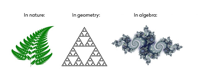
5. From nature to Timothy Leary in 3 small steps.

The patterns of agent diffusion within agent-based models could then be inferred as being
inherently representative of nature, natural process guided simply by the rules that naturally define our daily existence as defined by the automata and the demographics assigned to the agents within the agent-based model. The implications of all this fluff is that agent-based models can provide a good analogue for just that, natural process in addition to acting as an analytical tool to determine factors that may deviate those processes, providing an insight into the possible effects of affecting these processes with attenuating circumstances such as intense urbanisation, varying political climates and resource shortages; all key in the progression of human vulnerability and risk.

In terms of verification, envisage the situation where a flood is impending. You are broadly aware of flood policy and in the immediacy of impending situation you become aware of your neighbours beginning to leave their own homes or locale. Do you ask them why? Do you follow them? If so, why? If not, why not? Whatever your answers to this heavily loaded scenario may be, they will doubtlessly be littered with ‘ifs’ and ‘buts’ and this is fundamentally the obstacle policy faces in trying to ameliorate the fact that it is bound by more ‘ruban rouge’ than the Labour party directive on Brexit, is as apprehensible as the Voynich Manuscript and is as accessible as those two references compounded. Tools are required to test and visualise the compatibility interface between humans and policy before it is implemented. This will diversify and dilute it, making it more accessible; else it will forever be voided by its own hubris and lack of adequate testing. Whether the agent-based model can provide this panacea I am unsure, though one hopes.

An ode

So then, as this ode approaches the twilight of its purpose, having made it through the tour d’horizon of my research and personal interests, turgid with their own bias and logical fallacies (indicated at points, primarily to serve the author’s thirst for poetic liberty) I propose, a middle ground between pessimistic and optimistic bias, to the reader that you might embrace, and consider critically, the bias and fallacy that percolates through the world around you. In a world of climate change denial, where world leaders sharp-shoot their theses to inform decisions that affect us all and where it seems that technology and data has begun to determine our values and worth, it has never been more important to be self-aware and question the legitimacy of apathy for critique.

The ever-prescient Karl Popper suggested in his ‘conjectures and refutations’, that for science to be truly scientific a proposed theory must be refutable, as all theories have the potential to be ‘confirmed’ using the correct arrangement of words and data. It is only through refutation, or transcending the process of refutation, might we truly achieve progressive and beneficial answers to the questions upon which we base our theories. This being a process of empowerment and a sociological by-product of the positive freedom outlined by Erich Fromm. The freedom to progress collective understanding surely outweighs the freedom from fear of critical appraisal for having attempted to do so?  à chacun ses goûts, but consider this, in the final verse (7) of his Essay on Man, the final verse he ever wrote, Alexander Pope originally wrote that “One truth is clear, whatever is, is right.” By Popper’s standards, a lot of what ‘is’ today, shouldn’t be and this should ultimately leave us questioning the nature of our freedom, what exactly are we free to and free from? à chacun ses goûts?

‘All nature is but art, unknown to thee; 
All chance, direction, which thou canst not see; 
All discord, harmony, not understood; 
All partial evil, universal good: 
And, spite of pride, in erring reason’s spite, 
One truth is clear, whatever is, is right?
7. A section of the tenth (X) verse in the first epistle of Alexander Pope’s unfinished Essay on Man, (with edited last line for dramatic effect (1733-34.))
————————–
This blog was written by Cabot Institute member, Thomas O’Shea, a 2nd year Ph.D. Researcher at the School of Geographical Sciences, University of Bristol. His interests span Complex Systems, Hydrodynamics, Risk and Resilience and Machine Learning.  Please direct any desired correspondence regarding the above to his university email at: t.oshea@bristol.ac.uk.
Thomas O’Shea

Read Thomas’ other blog in this series:


Dadaism in Disaster Risk Reduction: Reflections against method

Grey Britain: Misery, urbanism & neuroaesthetics

The last time Earth was this hot hippos lived in Britain (that’s 130,000 years ago)

Image taken from Wikimedia Commons. Credit Paul Maritz.

It’s official: 2015 was the warmest year on record. But those global temperature records only date back to 1850 and become increasingly uncertain the further back you go. Beyond then, we’re reliant on signs left behind in tree rings, ice cores or rocks. So when was the Earth last warmer than the present?

The Medieval Warm Period is often cited as the answer. This spell, beginning in roughly 950AD and lasting for three centuries, saw major changes to population centres across the globe. This included the collapse of the Tiwanaku civilisation in South America due to increased aridity, and the colonisation of Greenland by the Vikings.

But that doesn’t tell the whole story. Yes, some regions were warmer than in recent years, but others were substantially colder. Across the globe, averaged temperatures then were in fact cooler than today.

To reach a point when the Earth was significantly warmer than today we’d need to go back 130,000 years, to a time known as the Eemian.

For about 1.8m years the planet had fluctuated between a series of ice ages and warmer periods known as “interglacials”. The Eemian, which lasted around 15,000 years, was the most recent of these interglacials (before the one we’re currently in).

Although global annual average temperatures were approximately 1 to 2˚C warmer than preindustrial levels, high latitude regions were several degrees warmer still. This meant ice caps melted, Greenland’s ice sheet was reduced and the West Antarctic ice sheet may have collapsed. The sea level was at least 6m higher than today.

Across Asia and North America forests extended much further north than today and straight-tusked elephants (now extinct) and hippopotamuses were living as far north as the British Isles.

How do we know all this? Well, scientists can estimate the temperature changes at this time by looking at chemicals found in ice cores and marine sediment cores and studying pollen buried in layers deep underground. Certain isotopes of oxygen and hydrogen in ice cores can determine the temperature in the past while pollen tells us which plant species were present and therefore gives us an indication of climatic conditions suitable for that species.

We know from air bubbles in ice cores drilled on Antarctica that greenhouse gas concentrations in the Eemian were not dissimilar to preindustrial levels. However orbital conditions were very different – essentially there were much larger latitudinal and seasonal variations in the amount of solar energy received by the Earth.

So although the Eemian was warmer than today the driving mechanism for this warmth was fundamentally different to present-day climate change, which is down to greenhouses gases. To find a warm period caused predominantly by conditions more similar to today, we need to go even further back in time.


The past 540 million years. Note the Eemian spike and the Miocene Optimum.
Glen Fergus / wiki, CC BY-SA

As climate scientists, we’re particularly interested in the Miocene (around 23 to 5.3 million years ago), and in particular a spell known as the Miocene-Climate Optimum (11-17 million years ago). Around this time CO2 values (350-400ppm) were similar to today and it therefore potentially serves as an appropriate analogue for the future.

During the Optimum, those carbon dioxide concentrations were the predominant driver of climate change. Global average temperatures were 2 to 4˚C warmer than preindustrial values, sea level was around 20m higher and there was an expansion of tropical vegetation.

However, during the later Miocene period CO2 declined to below preindustrial levels, but global temperatures remained significantly warmer. What kept things warm, if not CO2? We still don’t know exactly – it may have been orbital shifts, the development of modern ocean circulation or even big geographical changes such as the Isthmus of Panama narrowing and eventually closing off – but it does mean direct comparison with the present day is problematic.

Currently orbital conditions are suitable to trigger the next glacial inception. We’re due another ice age. However, as pointed out in a recent study in Nature, there’s now so much carbon in the atmosphere the likelihood of this occurring is massively reduced over the next 100,000 years.
——————————
This blog is written by Cabot Institute members Emma Stone, Research Associate in Climatology, University of Bristol and Alex Farnsworth, Postdoctoral Researcher in Climatology, University of Bristol.

This article was originally published on The Conversation. Read the original article.

Climate lessons from the past: Are we already committed to a warmer and wetter planet?

Last September, the Cabot Institute and the University of Bristol hosted the 2nd International Workshop on Pliocene Climate.   Following on from that, we have just  released a short video describing what the Pliocene is and its relevance for understanding climate change.

The Pliocene is a geological time interval that occurred from 5.3 to 2.6 million years ago.  This interval of Earth history is interesting for many reasons, but one of the most profound is that the Earth’s atmosphere apparently contained elevated concentrations of carbon dioxide – in fact, our best estimates suggest concentrations were about 300 to 400  ppm, which is much higher than concentrations of 100 years ago but lower than those of today after a century of intensive fossil fuel combustion.

Image by NASA

Consequently, the Pliocene could provide valuable insight into the type of planet we are creating via global warming.  Our video release happens to coincide with pronounced flooding across the UK and focussed attention on our weather and climate.  There is little doubt that increased carbon dioxide concentrations will cause global warming; instead, the key questions are: how much warming will there be and what are the consequences of that warming? One way to study that is to examine previous intervals of Earth history also characterised by high carbon dioxide concentrations. The comparisons are not perfect, of course; for example, during the Pliocene the continents were in roughly but not exactly the same positions that they are in today.  But it can serve as another piece of the puzzle in predicting future climate.

One of the key lessons from Earth history is climate sensitivity.  Climate sensitivity can be expressed in various ways, but in its simplest sense it is a measure of how much warmer the Earth becomes for a given doubling of atmospheric carbon dioxide concentrations.  This is well known for the Pleistocene, and especially the past 800,000 years of Earth history, an interval with detailed temperature reconstructions and carbon dioxide records from ice core gas bubbles.  During that time, and through multiple ice ages, climate sensitivity was about 2.5 to 3°C warming for a doubling of carbon dioxide, which is in the middle of the model-based range of predictions.

Ice core sampling.
Image by NASA ICE (Ice Core Vitals) [CC-BY-2.0]
Wikimedia Commons

Ice core records, however, extend back no more than a million years, and this time period is generally characterised by colder climates than those of today.  If we want to explore climate sensitivity on a warmer planet, we must look further back into Earth history, to times such as the Pliocene.  Reconstructing atmospheric carbon dioxide concentrations in the absence of ice cores is admittedly more challenging.  Instead of directly measuring the concentration of carbon dioxide in gas bubbles, we must rely on indirect records – proxies.  For example, carbon dioxide concentration influences the number of stomata on plant leaves, and this can be measured on ancient leaf fossils. Alternatively, there are a number of geochemical tools based on how carbon dioxide impacts the pH of seawater or how algae assimilate carbon dioxide during photosynthesis; these are recorded by the chemical composition of ancient fossils.

These estimates come with larger error bars, but they provide key insights into climate sensitivity on a warmer Earth.  Recent research indicates a convergence of Pliocene carbon dioxide estimates from these various proxies and gives us more confidence in deriving climate sensitivity estimates.  In particular, it appears that an increase of carbon dioxide from about 280 parts per million (the modern value before the industrial revolution) to about 400 parts per million in the Pliocene results in a 2°C warmer Earth. Accounting for other controls, this suggests a climate sensitivity of about 3°C, which confirms both the Pleistocene and model-based estimates.

It also suggests that we have yet to experience the full consequences of the greenhouse gases already added to the atmosphere.

So then, what was this much warmer world like?  First of all, it was not an inhospitable planet – plants and animals thrived.  This should not be a surprise; in fact, the Earth was much warmer even deeper into the past. The climate change we are inducing is a problem for humans and society, not our planet.

However, the Pliocene was a rather different world.  For example – and importantly, given current events in the UK –  these higher global temperatures were associated with a climate that was also wetter* than present.  That provides important corroborating evidence for models that predict a warmer and wetter future.

 Image by w:en:User:Ivan and licensed as GFDL

Perhaps most striking, sea level appears to have been between 10 to 40 metres  higher than today, indicating that both the Greenland Ice Sheet and  Antarctic Ice Sheet were markedly smaller.  To put that into context, the Met Office has already commented on how flooding in the UK has been and will be exacerbated by sea level rise of 12 centimetres over the last 100 years and a further 5 to 7 centimetres by 2030.

We must be careful in how we extract climate lessons from the geological record, and that is particularly true when we consider ice sheet behaviour.  One widely discussed concept is ice sheet hysteresis.  This is a fancy way of saying that due to feedback mechanisms, it could be easier to build an ice sheet on Greenland or Antarctica than it is to melt one.  If such hysteresis does stabilise our current ice sheets, then we should not assume a planet with 400 ppm of carbon dioxide will necessarily have sea level 20 metres higher than that of today. But if hysteresis is rather weak, then the question is not whether we will see massive sea level change but rather how long it will take (Note: It is likely to take centuries or millennia!).

Most importantly, the collective research into Earth history, including the Pliocene, reveals that Earth’s climate can change.  It also reveals that climate does not just change randomly: it changes when forced in relatively well understood ways.  One of these is the concentration of carbon dioxide in our atmosphere. And consequently, there is little doubt from Earth history that transforming fossil carbon into carbon dioxide – as we are doing today – will significantly impact the Earth’s climate system.

* See Brigham-Grette, J., Melles, M., Minyuk, P., Andreev, A., Tarasov, P., DeConto, R., Koenig, S., et al., 2013. Pliocene Warmth, Polar Amplification, and Stepped Pleistocene Cooling Recorded in NE Arctic Russia. Science 340 (6139), 1421-1427. doi: 10.1126/science.1233137 and Salzmann, U., Haywood, A.M., Lunt, D.J., 2009. The past is a guide to the future? Comparing Middle Pliocene vegetation with predicted biome distributions for the twenty-first century. Philosophical Transactions of the Royal Society A: Mathematical, Physical and Engineering Sciences 367 (1886), 189-204.

This blog is by Prof Rich Pancost, Director of the Cabot Institute.  Rich will be giving a public lecture on how biogeochemical cycles have regulated the global climate system throughout Earth’s history on 25 February in Bristol.  The event is free and open to all, do come along to learn more.

To learn more about the Pliocene – and palaeoclimate research, in general – you can watch Professor Gerald Haug’s public lecture, Climate and Societies, recorded at the Cabot Institute as part of the 2nd International Workshop on Pliocene Climate.

Prof Rich Pancost