Antarctica – Cabot Institute for the Environment blog

Frozen Empires revisited

Posted on February 1, 2021March 30, 2023 by janet.crompton

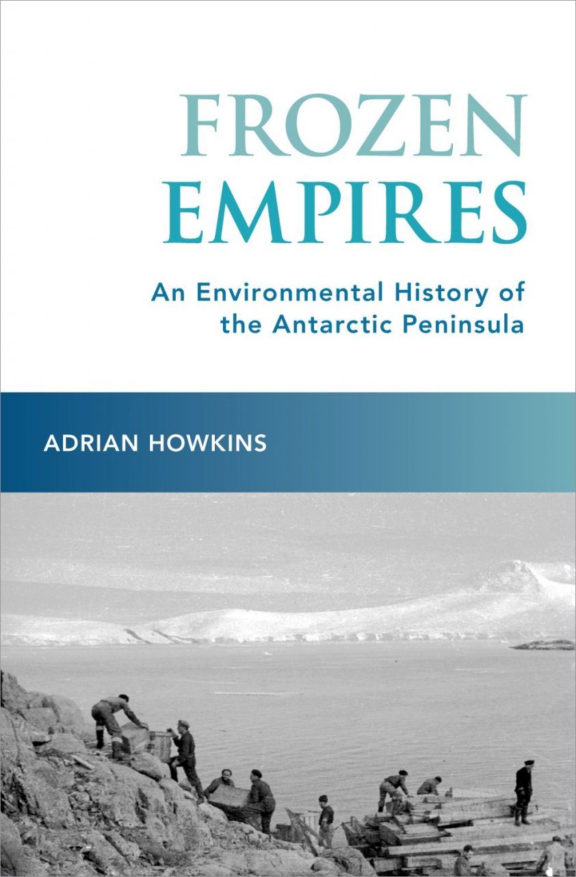
Image taken from the front cover of Adrian Howkin’s book – Frozen Empires

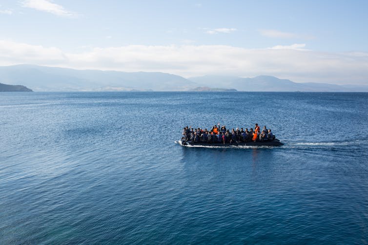
The recent release of the paperback edition of Frozen Empires: An Environmental History of the Antarctic Peninsula, offers an opportunity to revisit the arguments I made in this book and reflect on how it continues to shape my work in Antarctica and thinking about environmental history. The book sets out to frame the mid-twentieth century Antarctic sovereignty dispute among Argentina, Britain, and Chile as an environmental history of decolonization. Through a strategy I refer to as asserting ‘environmental authority’, Britain used the performance of scientific research and the production of useful knowledge to support its imperial claims to the region as a territory known as the ‘Falkland Islands Dependencies’. Argentina and Chile both contested Britain’s claim, and put forward their own assertations to sovereignty based on a sense that this was their environment as a result of proximity, geological contiguity, and shared climate and ecosystems. In the contest between British assertions of environmental authority and Argentine and Chilean ‘environmental nationalism’ it was the imperial, scientific vision of the environment that largely won out. There was no genuine decolonization of the Antarctic Peninsula region, or the Antarctic continent more generally. Instead, the 1959 Antarctic Treaty, which remains in force today, retains pre-existing sovereignty claims in a state of suspended animation (‘frozen’ in the pun of the treaty negotiators) and perpetuates the close connection between science and politics across the Antarctic Continent.

Much of my work since researching and writing Frozen Empires has focused on the history of the McMurdo Dry Valleys on the opposite side of the Antarctic continent. I am a co-PI on a US National Science Foundation funded Long Term Ecological Research (LTER) project, collaborating with scientists to ask how historical research might inform our understanding of this unique place. The McMurdo Dry Valleys are the largest predominantly ice-free region of Antarctica and since the late 1950s have become an important site of Antarctic science. Geologists are attracted to the Dry Valleys by the exposed rock, geomorphologists by the opportunity to study the glaciological history of the continent, and ecologists by the presence of microscopic ecosystems. The close connection between politics and science that I identified in the Antarctic Peninsula is also applicable to the history of the McMurdo Dry Valleys. The two most active countries in the region, New Zealand and the United States, can both be seen as making assertions of environmental authority to support their political position. A major difference is that now I find myself on the inside of this system, working with scientists to help produce the ‘useful information’ that is being used for political purposes.

Working as more of an insider in a system I critiqued in Frozen Empires raises a number of awkward questions. Can I retain a critical distance? Am I contributing to the perpetuation of an unequal system? What might the decolonization of Antarctic research look like? These questions are not easy to answer. Not infrequently I find myself looking back on the lack of inhibition I felt while researching and writing Frozen Empires and wishing for something similar in my current research. Academic collaboration by definition leads to entanglements, and these entanglements increase complexity. It is much easier, for example, to write critically about the imperial history of Antarctica than to convince scientific colleagues that this imperial history continues to have an impact on contemporary scientific research.

But for all the messiness and difficulties involved in collaboration, there are also tremendous opportunities. I have learned a lot about how science gets done through working with the McMurdo Dry Valleys LTER site, and I have learned about working as part of an academic team. Place-based studies offers an ideal opportunity for interdisciplinary research, and I think it is vital to have humanities perspectives represented in these collaborations. It takes time – often more time than expected – for effective collaborations to develop, and this process involves a significant degree of mutual learning. Researching and writing Frozen Empires fundamentally shaped what I bring to the table as an environmental historian in the McMurdo Dry Valleys project, and I remain convinced by its argument for imperial continuity. But the process of engaging in collaborative research has unsettled at least some of my earlier positions, and the book I’m writing on the history of the McMurdo Dry Valleys will likely be quite different to Frozen Empires.

—————————————-

This blog is written by Cabot Institute member Dr Adrian Howkins, Reader in Environmental History, University of Bristol.

It has been reposted with kind permission from the Bristol Centre for Environmental Humanities. View the original blog.

Frozen in time: reflections on a PhD and the history of Antarctica

Posted on April 20, 2020April 4, 2023 by janet.crompton

In March 2020, the third and final instalment of my PhD research made its way into Climate of the Past. In that article, I do my best to synthesise all I learnt over 5 years about an event that occurred 34 million years ago called the Eocene-Oligocene Transition. (Just so we are all on the same page: palaeoclimate scientists are interested in this period of the Earth’s history as it is when the first major Antarctic Ice Sheet appeared; before then Antarctica was warm and at least partially forested.)

An image of what Antarctica might have looked like at the onset of the Eocene-Oligocene Transition.

Four and a half years ago I wrote a piece for the Cabot Institute Blog about using a climate model to understand this point in the Earth’s history, and how many questions remained in our understanding. Why was the Earth so hot beforehand? What caused it to cool and eventually for Antarctica to glaciate? What other important changes would have occurred around the world at this time? At the time, I focussed particularly on the latter question.

The more time I spent trying to answer some of these questions, predictably (as is the way with science), the more complex some of them became. In the end, for my own peace of mind, I simply tried to bring together as much information as I could from lots of different sources to try to create a picture with some sort of clarity. I focussed on the high latitude Southern Hemisphere, because that is where a lot of the action was occurring at the Eocene-Oligocene Transition and it is also where models potentially have some difficulties in reproducing the climate.

To build up this picture, I used multiple climate model simulations of the period from two different modelling groups and compared these to the biggest dataset of proxy records of Southern Hemisphere climate 34 million years ago that I could compile by myself. Just reading and compiling all of the data from papers took me around a year. Not solidly (I had lots of other things to do too), but even still, reading papers solidly is very difficult in my opinion. Synthesising all of that different information into something coherent in my head is also something that I cannot force to happen quickly. It comes when it is ready.

Some of the complied proxy data for the high latitude Southern Hemisphere the Eocene-Oligocene Transition included in Kennedy-Asser et al. (2020).

In the end for this paper, I generated no primary data myself. It is all secondary data, either provided by other researchers I work with or taken from this very slow and lengthy review of scientific literature. Maybe, back at the start, that is not how I had pictured the finale of my thesis might look. Maybe the plan was to build up to some exceptional new result that I discovered, with data I produced with my own hands. But that wasn’t the case and, to be honest, I think it is better the way it is. Science is, and should be, a collaborative effort. In the spirit of this, I put all of the data I compiled and used, including all of my analysis scripts and detailed notes of where I obtained secondary data, up on the Open Science Framework. This way I hope the science can keep collaborating and continue growing.

Two thirds of my thesis were based on ‘my own’ data, messing around with a climate model, trying out new ideas, seeing if anything revolutionary popped out. This was really important too: for me to grow as a researcher, to learn about how the model works and to try to generate some outside-the-box ideas. Occasionally, of course, something truly revolutionary will be discovered. In the end, however, my conclusion is that model results often lack meaning by themselves: they need observations or proxy records to go with them to provide some sort of truth of what really happened, whether that is outside right now or 34 million years ago.

My new paper finds very similar things about why the Earth changed so much at the Eocene-Oligocene Transition to earlier research carried out nearly 20 years ago. It doesn’t challenge or rewrite everything we know, but that’s okay. The main scientific conclusion from my paper is that incorporating all of this data is actually essential to coming to the same conclusion as the research from many years ago. Without the inclusion of the boring, extensive data review, I might have quickly, excitedly jumped to a different conclusion that, on balance, seems less likely to be correct.

Much like this paper brings together different existing scientific data to compliment research built up over many years, it also brings together my own work and thoughts. It took many years, but it wouldn’t make sense to rush it: the conclusions take a bit of time, even if all of the data and answers are already out there.

————————————

This blog is written by Cabot Institute member Alan Kennedy-Asser, a Research Associate at the School of Geographical Sciences, University of Bristol. You can follow Alan on Twitter @EzekielBoom.

Alan Kennedy-Asser

Climate change: sea level rise could displace millions of people within two generations

Posted on June 4, 2019April 3, 2023 by janet.crompton

A small boat in the Illulissat Icefjord is dwarfed by the icebergs that have calved from the floating tongue of Greenland’s largest glacier, Jacobshavn Isbrae. Image credit: Michael Bamber

Antarctica is further from civilisation than any other place on Earth. The Greenland ice sheet is closer to home but around one tenth the size of its southern sibling. Together, these two ice masses hold enough frozen water to raise global mean sea level by 65 metres if they were to suddenly melt. But how likely is this to happen?

The Antarctic ice sheet is around one and half times larger than Australia. What’s happening in one part of Antarctica may not be the same as what’s happening in another – just like the east and west coasts of the US can experience very different responses to, for example, a change in the El Niño weather pattern. These are periodic climate events that result in wetter conditions across the southern US, warmer conditions in the north and drier weather on the north-eastern seaboard.

The ice in Antarctica is nearly 5km thick in places and we have very little idea what the conditions are like at the base, even though those conditions play a key role in determining the speed with which the ice can respond to climate change, including how fast it can flow toward and into the ocean. A warm, wet base lubricates the bedrock of land beneath the ice and allows it to slide over it.

Though invisible from the surface, melting within the ice can speed up the process by which ice sheets slide towards the sea. Gans33/Shutterstock

These issues have made it particularly difficult to produce model simulations of how ice sheets will respond to climate change in future. Models have to capture all the processes and uncertainties that we know about and those that we don’t – the “known unknowns” and the “unknown unknowns” as Donald Rumsfeld once put it. As a result, several recent studies suggest that previous Intergovernmental Panel on Climate Change reports may have underestimated how much melting ice sheets will contribute to sea level in future.

What the experts say

Fortunately, models are not the only tools for predicting the future. Structured Expert Judgement is a method from a study one of us published in 2013. Experts give their judgement on a hard-to-model problem and their judgements are combined in a way that takes into account how good they are at assessing their own uncertainty. This provides a rational consensus.

The approach has been used when the consequences of an event are potentially catastrophic, but our ability to model the system is poor. These include volcanic eruptions, earthquakes, the spread of vector-borne diseases such as malaria and even aeroplane crashes.

Since the study in 2013, scientists modelling ice sheets have improved their models by trying to incorporate processes that cause positive and negative feedback. Impurities on the surface of the Greenland ice sheet cause positive feedback as they enhance melting by absorbing more of the sun’s heat. The stabilising effect of bedrock rising as the overlying ice thins, lessening the weight on the bed, is an example of negative feedback, as it slows the rate that the ice melts.

The record of observations of ice sheet change, primarily from satellite data, has also grown in length and quality, helping to improve knowledge of the recent behaviour of the ice sheets.

With colleagues from the UK and US, we undertook a new Structured Expert Judgement exercise. With all the new research, data and knowledge, you might expect the uncertainties around how much ice sheet melting will contribute to sea level rise to have got smaller. Unfortunately, that’s not what we found. What we did find was a range of future outcomes that go from bad to worse.

Reconstructed sea level for the last 2500 years. Note the marked increase in rate since about 1900 that is unprecedented over the whole time period. Robert Kopp/Kopp et al. (2016).

Rising uncertainty

We gathered together 22 experts in the US and UK in 2018 and combined their judgements. The results are sobering. Rather than a shrinking in the uncertainty of future ice sheet behaviour over the last six years, it has grown.

If the global temperature increase stays below 2°C, the experts’ best estimate of the average contribution of the ice sheets to sea level was 26cm. They concluded, however, that there is a 5% chance that the contribution could be as much as 80cm.

If this is combined with the two other main factors that influence sea level – glaciers melting around the world and the expansion of ocean water as it warms – then global mean sea level rise could exceed one metre by 2100. If this were to occur, many small island states would experience their current once-in-a-hundred–year flood every other day and become effectively uninhabitable.

A climate refugee crisis could dwarf all previous forced migrations. Punghi/Shutterstock

For a climate change scenario closer to business as usual – where our current trajectory for economic growth continues and global temperatures increase by 5℃ – the outlook is even more bleak. The experts’ best estimate average in this case is 51cm of sea level rise caused by melting ice sheets by 2100, but with a 5% chance that global sea level rise could exceed two metres by 2100. That has the potential to displace some 200m people.

Let’s try and put this into context. The Syrian refugee crisis is estimated to have caused about a million people to migrate to Europe. This occurred over years rather than a century, giving much less time for countries to adjust. Still, sea level rise driven by migration of this size might threaten the existence of nation states and result in unimaginable stress on resources and space. There is time to change course, but not much, and the longer we delay the harder it gets, the bigger the mountain we have to climb.

Click here to subscribe to our climate action newsletter. Climate change is inevitable. Our response to it isn’t.

This blog was written by Cabot Institute member Jonathan Bamber, Professor of Physical Geography, University of Bristol and Michael Oppenheimer, Professor of Geosciences and International Affairs, Princeton University. This article is republished from The Conversation under a Creative Commons license. Read the original article.

Antarctica: Looking back

Posted on May 11, 2019April 13, 2023 by janet.crompton

Back on dry land after seven-and-a-half weeks at sea, the sights of the Southern Ocean are already drifting from my mind into the whirlwind of modern life. The threats of land-sickness never materialised and the taste of fresh fruit and vegetables is everything I hoped it would be. Reflecting on a research cruise is not dissimilar to reflecting on a PhD.

“We only remember half”

Looking back can be a glorious thing. We all know the benefits that hindsight can bring. There are few things in our lives we couldn’t improve, whether they be things we said, research we carried out or ideas we had, if we got but one trial run at everything first. But looking back also gives the past a magical quality. The vividness of a blue sky intensifies, the significance of a rare sight swells and all the hardships are suppressed into one dense ball that our mind tries not to remember. The retelling of tales reconsolidates the good memories at the expense of the bad.

Of course this isn’t always the case and, if we really take the time, all of the gory details can be unpacked. I’m reading an amazing book at the moment, The Worst Journey in the World by Apsley Cherry-Garrard, that gives the most warts-and-all description of early Antarctic exploration. His descriptions are detailed, his wit hilarious and his tale harrowing. He is one of three who dragged two sleds to an emperor penguin colony in the heart of the Antarctic winter, being physically frozen into their clothes, losing their tent to a blizzard and of course getting plenty of frostbite. They did this just to collect three penguin eggs for science, as they hoped the embryos could be used to shed light on the evolutionary history of these creatures, which they believed were more primitive than other birds. The following year several of his closest friends died on the return leg of making it to the South Pole with Scott and he had to help recover their bodies.

Needless to say, Apsley didn’t have the greatest time in Antarctica, but still he writes:

Whatever merit there may be in going to the Antarctic, once there you must not credit yourself for being there. To spend a year in the hut at Cape Evans because you explore is no more laudable than to spend a month at Davos because you have consumption … It is just the most comfortable thing and the easiest thing to do under the circumstances.

This book is a definitive grim account of fieldwork and I really had nothing to complain about during our research cruise. To rephrase Apsley:

The [James Clark Ross], as [ships] go, was as palatial as is the Ritz, as hotels go.

A few nods towards monotony in work and some bad nights’ sleep in the previous blog articles in this series are all the negative memories I need to keep, otherwise the rest can go down for the record as one of the most interesting experiences of my PhD.

Southern Ocean Bridgeman Island Bridgeman Island off the Antarctic Peninsula. The sea was a bit choppy that day, but nothing too major to complain about.

Questions remain

I have just completed my PhD viva and, pending some minor corrections to my thesis, I have drawn a line under a four-and-a-half-year period of my life. During that time, most of my intellectual energy has gone into trying to understand what Antarctica was like in the past. Despite having been situated more or less in the same position over the South Pole for over 100 million years, this continent twice the size of Australia hasn’t always been the cold, inhospitable place that Apsley and co. experienced so brutally.

Fossils found on the few exposed outcrops of rock around the coast of the continent, on the sub-Antarctic islands and in the Transantarctic mountain range that cuts across between the Weddell and Ross Seas, show that up until relatively recently, diverse vegetation lived on this continent. (By relatively recently, I mean up until potentially 5 million years ago or so.) Definitely up until the end of the Eocene (the period I researched), much of the continent is believed to have been ice free.

The past environment of the Earth can be reconstructed using all sorts of complex chemistry and dating of past rocks and sediments, but the simplest and sometimes most compelling evidence can be those geological indicators that can be seen with the naked eye. Fossilised leaves, branches and seed pods from a variety of Southern Beech, most similar to modern Nothofagus Antarctica, show quite clearly what kind of ecosystem used to exist.

Nothofagus Antarctica and the Magellanic Forest, Southern Chile: a window into the past environment of Antarctica?

Nothofagus Antarctica and the Magellanic Forest, Southern Chile: a window into the past environment of Antarctica?

Today, Southern Beech forests can be found in Patagonia and other high latitude regions of the Southern Hemisphere. On our one day off we had in Punta Arenas before we set sail, I went with the other researchers from Exeter up into the Magellanic Forest Park just outside the town. As we walked through this ancient forest, snarled up in Old Man’s Beard lichen, with birds singing on a warm, sunny autumn day, I had to think ‘So this is what I (and lots of other people) have said Antarctica might have been like 34 million years ago?’

My research uses climate models to try to understand the processes that could explain the geological evidence of past climate. While there are some things they can help us understand reasonably well, there are other aspects of the Earth system that still remain difficult to explain, even after decades of research. How could the Earth remain warm enough to sustain forests over Antarctica and not freeze up? That is one such question which I can’t definitively answer.

My PhD research also focussed a lot on the importance of deep water formation on the regional temperatures in the Southern Ocean around the end of the Eocene. There could be little fieldwork more relevant therefore than going to try to understand deep water formation occurring around Antarctica today. Through conversations with researchers from all over the UK and beyond on the many long days of the cruise, I got an insight into the uncertainties that still exist in understanding this process today. Compared to the observational data we collected on our cruise, I looked at how the climate model we use compares in how it recreates the present day ocean. While there are some realistic elements, there are also some important differences which have planted future research questions in my brain. If these are the uncertainties in the model for the present day, how uncertain might my simulations of the ancient world be?

Crabeater seal in Antarctic pack ice. Understanding deep water formation remains challenging, in part because of how extreme the environment is.

Terra Australis Incognita

Looking back isn’t always easy. The deeper back in time we try to look, the harder it becomes to find data and to synthesise it with our knowledge of how the Earth and its oceans, atmosphere and biology work. In writing my PhD thesis, I had to come to terms with not knowing all of the answers. There are many, many questions that are too big and too complex to solve even with years of effort and 50,000 words. Stepping onto the James Clark Ross reminded me of that fact like a blast of 40 knot southerly Antarctic air to the face.

In the 17th Century, cartographers grappled with their limited understanding of this world, putting together the pieces of information they had and using artistic license to fill in the unmapped gaps that explorers had yet to reach. This map by Blaeu includes the Terra Australis Incognita, or ‘Unknown Southern Land’. While modern science would generally not approve of such guess work, exploring the history of the Earth system is a similar step into the unknown, with geologists, palaeoceanographers and palaeoclimatologists having to build the picture around what limited information they have.

A section of map by Blaeu (1645-1646), showing the as yet uncharted and hence imagined Terra Australis Incognita. Image courtesy of Special Collections, University of Bristol Library.

From 1646, when Blaeu’s map was published, it was a further 174 years before the first humans saw the Antarctic continent. Now, nearly 200 years on from that first sighting, the Unknown Southern Land still holds many secrets.

Still, looking back also shows how far we have come: a pleasant relief from thinking how far we have yet to go. We know so much more about Antarctica today than we ever have. Unfortunately, with hindsight, Apsley and co.’s journey to find emperor penguin eggs in the middle of winter was a relatively fruitless exercise as the hypothesis they were collecting the eggs to test has since been proven wrong: emperor penguins are actually very specialised and highly evolved birds, not primitive or reptile-like.

Should we give up because we might never know the answers or we might be going down a blind alley? I don’t think so. I’ll give the last words to Apsley, as he really, really earned them.

The question constantly put to us in civilization was and still is: ‘What is the use? Is there gold? Or is there coal? … The members of this expedition believed that it was worthwhile to discover new land and new life, to reach the Southern Pole of the Earth, to make elaborate meteorological and magnetic observations and extended geological surveys … They were prepared to suffer great hardship; and some of them died for their beliefs. …We travelled for science … in order that the world may have a little more knowledge, that it may build on what it knows instead of on what it thinks.

Apsley Cherry-Garrard in The Worst Journey in the World

———————————–

This blog is part of a blog series from Antarctica by Alan Kennedy-Asser, who has recently completed his PhD at the University of Bristol. This blog has been republished with kind permission from Alan. View the original blog. You can follow Alan on Twitter @EzekielBoom.

Alan Kennedy-Asser

Read part one of Alan’s Antarctica blog series – Antarctica: Ship life
Read part two of Alan’s Antarctica blog series – Antarctica: Why are we here again?
Read part three of Alan’s Antarcica blog series: Antarctica: Looking back

Antarctica: Why are we here again?

Posted on April 8, 2019April 13, 2023 by janet.crompton

The ship’s roll reaches 19° and everything falls off the desk, nearly followed by me off my chair if it weren’t for an evasive leap to one side. My roommate wakes with a start as the curtains around his bed have flung themselves open. “What are you doing?” he asks, in a confused state. Aside from the fact that everything falling off the desk was the weather’s fault, not mine, his question is a good one.

What are a team of 20 scientists, mostly from the UK, doing out here in the Southern Ocean? Surely there’s somewhere closer to home we could measure the sea. The main aim of this research cruise is to understand the process of deep water formation around Antarctica. First, let me briefly explain what deep water formation is and why it’s important in about 300 words. To understand this, the most important thing to remember is that water becomes denser when it is colder and/or when it is saltier. I think they teach that in GCSE science; if they don’t, they should.

Deep water formation

Antarctica is pretty cold, obviously. Where we are now, the sea temperature is around 1 °C. If we were to go further south or wait until winter, the sea will approach its freezing point of around -2 °C, forming sea ice. That’s a little colder than normal water, which freezes at 0 °C, because the sea is salty. However, when the sea freezes to form sea ice, the salt from the water is not incorporated into the ice – the salt that was in the sea water is left behind, making the remaining water a little bit saltier. As a result, the water close to the sea ice edge is both cold and salty compared to the rest of the world’s oceans, and therefore is denser than most of the rest of the world’s oceans. Dense water sinks below less dense water, and so the deepest water at the bottom of the oceans around the world all comes from around Antarctica.

Sea ice drifting close to the tip of the Antarctic Peninsula

When the water is at the surface of the sea, it can absorb heat and gases, including carbon dioxide, from the atmosphere. When deep water formation occurs, this heat and carbon dioxide can be drawn down into the depths of ocean, where it will stay for 1000 years or so. The research cruise I am on now wants to measure the amount of deep water formation occurring so we can better understand how much heat and carbon dioxide is being taken up by the ocean, which helps understand how much the climate will change in the future with global warming. That’s why we are here, basically, instead of the Bristol Channel.

Chlorofluorocarbons

Our team, based at the University of Exeter, are specifically measuring CFCs in the water. CFCs (chlorofluorocarbons) are manmade gases that were used for many industrial and commercial processes for a few decades before people realised they were destroying ozone in the atmosphere. This was creating a hole in the Earth’s ozone layer in the stratosphere over Antarctica and the Southern Hemisphere. Ozone is important for absorbing some of the Sun’s strong and damaging ultraviolet radiation before it reaches the Earth’s surface. Excessive ultraviolet radiation causes sunburn and skin cancer in humans, so people were concerned about the ozone hole when it was discovered in the 1980s. As a result, all nations of the world agreed the Montreal Protocol to stop producing CFCs that were destroying the ozone layer. Although this was a geopolitical and diplomatic success story, the ozone hole is only slowly showing signs of recovering and some CFCs still seem to be increasing (presumably suggesting some illegal production of them still occurs). However, luckily the ozone hole is no longer getting bigger and it is mostly contained to the very high Southern Hemisphere. Don’t worry, I brought plenty of factor 50 for my pasty Irish skin.

The reason we are measuring CFCs, however, is not actually to understand what they are doing to the ozone layer. We care about CFCs because they are manmade gases that are not naturally found in the atmosphere or ocean. This allows them to be used to trace ocean circulation and processes such as deep water formation. Let me explain how.

Jetsam

Since setting off from the Falklands five weeks ago, we have seen two manmade things: a ship on the horizon and some rusty metal oil barrels floating around amongst a heavy scattering of icebergs. The ship was a fishing boat, not far from the Falklands or Punta Arenas, so was not too surprising. The oil barrels however, were a bit more unexpected. They were floating right in the middle of the Weddell Sea, almost as far from civilisation as they could be. There were at least four of them, however they weren’t lashed together like some sort of raft made by Tom Hanks, they were all floating individually within a few hours steam of each other.

Oil barrel floating in the Weddell Sea, originally dumped around 6,000 km away (image credit: Hugh Venables, BAS)

The most curious thing about these barrels, however, is that when we were able to zoom in on a photo taken of one with a camera with a good telephoto lens, we could see their origin. They had writing and the branding from Operation Deepfreeze, a US mission to set up an Antarctic base in the Ross Sea in the 1950s. After initially being surprised at seeing any litter in the pristine Southern Ocean, we had to question how these barrels got here. The Ross Sea is on the entire other side of the Antarctic continent, around 6,000 km away by sea.

The Operation Deepfreeze base was built on the Ross Ice Shelf. This is thick ice that has flown out from the glaciers on land to create an area the size of France floating over the Ross Sea. Although this ice is very thick and reasonably slow moving, it is not permanent and does break off from time to time to form huge icebergs. The same process has formed some icebergs that have made the news recently, including one berg a quarter of the size of Wales and a potential berg break off that is threatening to take the British Antarctic Survey’s Halley research station with it. Well, presumably the old dumping ground from Operation Deepfreeze has at some stage broken off from the Ross Ice Shelf, floated halfway around the Southern Ocean carried by the Antarctic Circumpolar Current and been taken into the Weddell Sea gyre, where it melted and broke up, scattering all the rubbish into the Weddell Sea.

Just like these oil barrels can be used to trace how the ocean’s surface currents circulate (a similar story involves a spilt shipping container of rubber ducks in the Pacific Ocean in 1992), looking at where manmade gases such as CFCs end up in the deep ocean can tell us how the deep water formation takes water from the surface to depth. To measure the CFCs, we first take samples using a probe known as a CTD (which stands for Conductivity Temperature Depth). This probe has 24 bottles on it as well as instruments for measuring of salinity, temperature and other water properties. The probe is lowered to the bottom of the ocean (which around here can be more than 6 km deep) and as it is brought back up to the surface, the 24 bottles are closed at different depths. When the CTD arrives back on the ship’s deck, we then have samples of water from 24 depths through the ocean at that particular location. Over the course of the cruise, we will be carrying out around 100 CTDs.

Sampling using the CTD (lowered by winch off the side of the ship) continues morning, noon and night, meaning we work 12 hour shifts

With the water brought up in the bottles, our team takes a 500 ml sample from each and we store them in a walk-in fridge on the ship. We then analyse one sample at a time, which takes about 20 minutes using a custom-built machine that strips all the gases out of the water and calculates the amount of CFCs it contains. This setup for measuring CFCs is in its own portable lab, built in a shipping container that it strapped onto the aft deck of the James Clark Ross. While it’s pretty time-consuming running 100 CTDs with 24 bottles each taking 20 minutes (I calculate that to be more than 33 days of continually running the machine, assuming no delays) at least we have a good view from our container out over the wildlife and icebergs of the Southern Ocean.

Our CFC lab inside a shipping container, strapped onto the aft deck, as we sail by the South Orkney Islands

Other science

Besides our team measuring CFCs, other scientists are also using the water from the CTD to analyse oxygen isotopes, nutrient content, pH and microbes. When the CTD comes on deck, there is usually a bit of a mad scramble as everyone gets water for their own analysis, with a strict pecking order as who gets to take their water first. For maximum inconvenience, usually the CTD comes up just before dinner or lunch, just to make sampling that little bit more frantic.

Taking water samples for analysis from the 24 bottles on the CTD once it is back on deck (image credit: Charel Wohl, PML)

As well as measuring water from depth using the CTD, other scientists on the ship also continually measure the air and surface sea water as we sail. The air measurements, taken from the very front of the ship so not to get contaminated by exhaust or air conditioning fumes, must be measuring some of the cleanest air in the world. It’s pretty nice to stand up there and breathe it in, although it’s often accompanied by a blizzard of snow and biting wind, which makes the experience slightly less enjoyable.

We also have deployed some floats that will continue to measure the salinity and temperature of the sea here for the next five years or so. Using a gas bladder, these floats can adjust their density so they rise and sink through the ocean, measuring continually as they go. Every time these floats get back to the surface, they send their data back via a satellite connection. Although they don’t measure as much stuff as the scientists on the ship (for example, they don’t measure CFCs), they will be here all year round so keep making measurements through the winter. The ship on the other hand will have to retreat from the sea ice before the winter sets in, in case we end up repeating Shackleton’s antics with the Endurance. Which is fine with me because, interesting as it is, I don’t really fancy a further 6 months down here in the dark.

A float being deployed, which will continue to make measurements through the winter and for years after we leave

——————————————-
This blog is part of a blog series from Antarctica by Alan Kennedy-Asser, who has recently completed his PhD at the University of Bristol. This blog has been republished with kind permission from Alan. View the original blog. You can follow Alan on Twitter @EzekielBoom.

Alan Kennedy-Asser

Antarctica: Ship life

Posted on March 25, 2019April 13, 2023 by janet.crompton

The RRS James Clark Ross docked in the Falkland Islands

Blinking blurry eyes, I crack open the curtains and gaze out into the bright light of a new day. A hulking white and blue iceberg gazes back at me. Even after a broken night’s sleep being shunted from one side of my bunk to the other as the ship bounces through swell, that still makes a rewarding start to each day. Through an unexpected turn of events, I’ve found myself on the British Antarctic Survey’s RRS James Clark Ross, on a seven-week long research cruise helping researchers from the University of Exeter take samples and measure CFCs in the Weddell Sea. Having just handed in my PhD thesis – after four years of studying and researching Antarctic climate and hearing the question “do you get to go to Antarctica?” countless times – the opportunity to help out on this cruise was too good an opportunity to pass up. Life on a ship gives you plenty of time to think (and write), but I promise to keep these musings brief in three posts: ship life; the science and why we’re here; and how the real thing compares to a PhD.
—————————————-
This is my first experience of life on a ship. Previously, my most extensive experience of boat life was the eight hours on the Stena Line from Liverpool to Belfast, so I shall use that as my reference frame. Stena Line regularly ask you to fill out feedback forms and rate your experience to have the chance to win back the cost of your trip, so I shall do the same here (although as usual I don’t expect to win anything).

How did you find the booking procedure?

Stena Line have a fast and efficient website for making and managing bookings. Signing up for the research cruise was also pretty straight forward, although that was likely aided by me having done a PhD in Antarctic-related science and knowing someone at the British Antarctic Survey (BAS) who forwarded me the advert. I emailed the lead scientist from Exeter saying I was interested, we had a chat on Skype then I had to confirm that my PhD supervisors at Bristol were happy for me to go.

Generally, however, beyond that point there was a bit more faff than booking the Stena Line. BAS require quite a few forms filling out, some of which require a bit more homework, including passing a medical examination and a sea survival course. The authentic personal sea survival certificate had to be presented on getting on the boat before sailing. In contrast, the Stena Line rarely even ask for ID (although I suppose this might change after Brexit).

Stena Line: 5/5
James Clark Ross: 3/5

How did you find the check-in procedure?

The check-in for the Stena is remarkably simple, and as mentioned they rarely even ask for ID. Getting onto the James Clark Ross was logistically more complicated, requiring flights from Heathrow to Madrid, Madrid to Santiago in Chile, and Santiago to Punta Arenas. Although this journey took more than 24 hours, I still preferred it to driving in the rain up the M5 and M6 from Bristol, as I got free food and could watch films. Punta Arenas is also nicer than Birkenhead and I found the language barrier easier to overcome in Chile (Scouse can be very confusing at times).

Stena Line: 3/5
James Clark Ross: 4/5

Exploring the Magellanic forest above Punta Arenas

How did you find the cabins (if applicable)?

Getting a cabin on the Stena Line is not necessary, particularly if travelling during the day time sailing. The last time I travelled on the night time crossing, however, the cabin was not overly satisfactory with uncomfortable beds, an unclean bathroom and a broken soap dispenser. Stena customer services subsequently refunded the cost of the cabin. On the James Clark Ross, the cabins are slightly smaller than the Stena Line, however, there is ample storage space, the beds are pretty comfortable and there are privacy curtains for each bunk, which is good when you are on slightly different work shifts to your roommate. The biggest complaint about the James Clark Ross is that it makes many strange noises and rocks a lot more in the heavy weather, which can keep you up a lot of the night. These noises include a high-pitched wail which is either the stabiliser system or sirens luring us to our watery graves. The latter seems more likely.

Stena Line: 1/5
James Clark Ross: 3/5

How did you find the food onboard?

The Stena’s Met Grill is renowned for its fried breakfast and hearty lunch and dinner menu. The portion sizes are good, however, the prices are also a bit steep. On the James Clark Ross, three square meals a day are available (including midnight dinner service for those on night shifts), with lunch and dinner both offering 3+ courses. Because of how my shift patterns work out, it doesn’t make sense to get up for breakfast, so I just eat a 3-course lunch and dinner each day. Remarkably, over 4 weeks since we left, there is still fresh fruit and some salad on the go. The variety has been good, and they also have included some of the classics off the Stena Line menu, including fish and chips (most Fridays), curry (every Saturday) and Swedish meatballs. Although I have also had Swedish meatballs on the Stena, I have never tried authentic (Ikea) Swedish meatballs to know which is closer to the real deal.

Stena Line: 4/5
James Clark Ross: 5/5

How did you find the onboard shopping?

The shop onboard the Stena Line is pretty awful. They sell head phones if you forgot yours, which is about the only thing I have ever bought from it. They also sell some magazines and over-priced toys in case you didn’t realise the crossing was 8 hours and find yourself going slightly insane. The shop on the James Clark Ross, called the bond, is stocked with James Clark Ross branded clothing, toiletries, chocolate bars and some odds and ends like postcards and plaques. Unfortunately, as the ship is nearing the end of its working life for BAS, being replaced next year by the RRS Sir David Attenborough (of Boaty McBoatface fame), none of the branded clothing is being restocked. That means the only things that are left are in sizes XXL or age 7-8, neither of which are much use to me.

Stena Line: 1/5
James Clark Ross: 1/5

How did you find the onboard entertainment and facilities?

Both ships have a bar. The James Clark Ross bar is extremely cheap, however, many of the beers are about six months past their best before dates, which can result in ‘bowel roulette’ the following day. A worthwhile sacrifice if you’re unemployed like me. The lounge area is remarkably similar between both boats and is comfortable enough. The internet connection is much better on the Stena, although they possibly harvest your personal data in the process of providing it. On the James Clark Ross, they have to commit some of the internet to facilitate the science (boring), so the bandwidth for personal connections is not as strong.

Besides the gambling machines, the Stena Line’s main attraction is the cinema, which can be good if they have a decent film being shown. On the James Clark Ross, although they do not have a dedicated cinema room, they have a huge selection of DVDs and an endless supply of films available on people’s laptops which can all be put through a projector. There are also loads of board games and a few musical instruments onboard too, which are nice to have a jam on and facilitated a St Patrick’s Day gig and ceilidh dance. Although the James Clark Ross has a greater range of entertainment available, the Stena Line only has to keep you amused for 8 hours, not 7 weeks, so this one is a tight run context. Luckily when you have to work 12 hour shifts, you don’t have much time for entertainment.

Stena Line: 3/5
James Clark Ross: 4/5

St Patrick’s Day decorations in the bar

Would you recommend this crossing to a friend?

Usually my answer to this is ‘yes’ for the Stena Line. It’s a handy way of getting to England from Belfast, saving the drive through North Wales and up from Dublin. Admittedly there’s not much to see in the Irish Sea except the odd shearwater and the Isle of Mann, but generally the crossing is smooth because of the size of the ship (around 185m long) even when the weather is bad. On the James Clark Ross, the research cruise route very much agrees with the old saying ‘The adventure is in the journey, not the destination’. We are analysing a transect through the Southern Ocean and Weddell Sea and end at 57.5°S, 30°E, which is precisely in the middle of nowhere (go ahead and look it up on Google Maps). Although we don’t end anywhere in particular, the route has been spectacular at times: we’ve sailed past a number of sub-Antarctic islands, countless colossal icebergs, seen penguins on land, in the sea and on ice, had dolphins, fin whales, and humpbacks right by the ship (the latter breaching dramatically at times) and had regular, effortless fly-bys from wandering albatrosses and other seabirds great and small. The weather has been mixed and as the ship is 100m long it feels the swell a bit more than the Stena, however, the seas so far have been much more merciful than I had expected.

Humpbacks taking a breath, Coronation Island, South Orkneys

As exciting as it is to see the Isle of Mann and the Mourne Mountains, on the whole, I would say Antarctica just about tops the Irish Sea. Sorry Stena Line. Although, for health and safety reasons I’m sure the crew of the Stena Mersey are happy enough to not have to dodge all of these icebergs.

Stena Line: 4/5
James Clark Ross: 5/5

—————————–
This blog is part of a blog series from Antarctica by Alan Kennedy-Asser, who has recently completed his PhD at the University of Bristol. This blog has been republished with kind permission from Alan. View the original blog. You can follow Alan on Twitter @EzekielBoom.

Alan Kennedy-Asser

Atmospheric and oceanic impacts of Antarctic glaciation across the Eocene–Oligocene transition

Posted on October 8, 2015April 13, 2023 by janet.crompton

Composite satellite image of what the Earth may have looked like prior to Antarctic
glaciation during the late Eocene (image by Alan Kennedy).

The Eocene-Oligocene Transition occurred approx. 34 million years ago and was one of the biggest climatic shifts since the end of the Cretaceous (with the extinction of the dinosaurs). The Earth dramatically cooled and the Antarctic ice sheet first formed, but the cause and nature of the cooling remain uncertain. Using a climate model, HadCM3L, we looked at the effect of ice sheet growth and palaeogeographical change (i.e. continental reconfiguration as Australia separated from Antarctica) on the Earth’s steady-state climate. We utilised four simulations: a late Eocene palaeogeography with and without an ice sheet and an early Oligocene palaeogeography with and without an ice sheet.

The formation of the Antarctic ice sheet causes a similar atmospheric response for both palaeogeographies: cooling of the air over Antarctica, intensification of the polar atmospheric cell and increased winds over the Southern Ocean. The sea surface temperature response to the growth of ice is very different, however, between the two palaeogeographies. For the Eocene palaeogeography there is a 6°C warming in the South Pacific sector of the Southern Ocean in response to ice growth, but very little change (or even a slight cooling) for the Oligocene palaeogeography. Why, under the same forcing (the appearance of the ice sheet), do these different palaeogeographies have such different sea surface temperature responses?

The stronger winds over the Southern Ocean force more-saline water from the southern Indian Ocean into the less-saline southern Pacific Ocean. This is particularly important for the Eocene simulations, where the narrow gap between Australia and Antarctica limits flow from the Indian to the Pacific Ocean. As salinity in the southern Pacific Ocean increases the water becomes denser and sinks, releasing heat. This accounts for the increase in sea surface temperature in the Eocene simulations. In the Oligocene simulations, flow is already much greater between the Indian and Pacific Oceans, and so there is no marked increase in density, sinking or sea surface temperature following glaciation. There is only a mild cooling due to the presence of the large, cold ice sheet.

Whether in reality the dominant ocean response to glaciation was warming or cooling may have impacted the growth of the ice sheet at this major transition in the Earth’s history. However, more importantly, this research highlights that sensitivity to subtle changes in palaeogeography can potentially have very large effects on the modelled climatic response to an event such as Antarctic glaciation. This could be very important for understanding palaeoclimate records and interpreting climate model results.

This research, carried out by Alan Kennedy, Dr Alex Farnsworth and Prof Dan Lunt of the Cabot Institute and University of Bristol with others, is featured in a special issue of the Philosophical Transactions of the Royal Society A. The full special issue on the theme of ‘Feedbacks on climate in the Earth System’ and the paper can be accessed here.

Special issue cover (image from Royal Society).

Citation: Kennedy A.T., Farnsworth A., Lunt D.J., Lear C.H., & Markwick P.J. (2015) Atmospheric and oceanic impacts of Antarctic glaciation across the Eocene–Oligocene transition. Phil. Trans. R. Soc. A, 373, 20140419, doi:10.1098/rsta.2014.0419.
—————————-
This blog is written by Alan Kennedy from the School of Geographical Sciences at the University of Bristol. This blog post was edited from Alan’s blog post at Ezekial Boom.

Alan Kennedy

Uncertain World: Understanding past and future sea level rise

Posted on September 25, 2015April 13, 2023 by janet.crompton

A recent study published in Science Advances suggests that if we burn all attainable fossil fuels (up to 12,000 gigatonnes of carbon), the Antarctic ice sheet is likely to become almost ice-free within 10,000 years. However, what does this mean in terms of sea level rise? To illustrate this we have designed an infographic which shows the likely extent of sea level rise under a range of different scenarios. We have chosen to use the Wills Memorial Building as an example and assume, for the purpose of this exercise, that it resides at sea level (Figure 1).

1) Sea level rise over the next century:

The most recent report by the Intergovernmental Panel on Climate Change (IPCC AR5) indicates that if we continue emitting greenhouse gases under business-as-usual scenarios (i.e. no reduction in emissions), it is likely that global mean sea level will rise between 0.52 and 0.98 m by the year 2100. If we are more optimistic, and we allow greenhouse gas emissions to peak in 2040 and decline thereafter, the range of likely global mean sea level rise is lower, but not insignificant (0.36 to 0.71 m). Both of these estimates are illustrated below and shown alongside the Wills Memorial Building.

Figure 1: An infographic showing the approximate height of sea level rise depending upon a range of different scenarios (Fretwell et al., 2013; IPCC AR5). This assumes the Wills Memorial Building resides at sea level

Although ~30 to 100 cm of sea level rise may seem insignificant, it is worth considering what this means for other regions. For example, “…since 80% of its 1,200 islands are no more than 1m above sea level“, sea level rise has the potential to impact up to 360,000 citizens and lead to widespread migration.

The reason that scientists provide a range of values for sea level rise is that the climate system is very complex. For example, under low emissions scenarios, there is expected to be an increase in moisture content around Antarctica, leading to increased snowfall along the ice sheet margins. However, under higher emissions scenarios, ice sheet discharge overcompensates for an increase in snowfall, leading to a net sea level rise.

2) Sea level rise over 10,000 years:

The variations between these two emission scenarios are less important when looking over longer timescales. Winklemann et al. (2015) have recently simulated changes in the Antarctic ice sheet over the next 10,000 years using a combination of climate and ice sheet models. From these experiments, it is clear that ice loss is driven by two key feedback mechanisms. The first begins with warming and subsequent retreat of the grounding line (Figure 2). The grounding line is the region where ice transitions from a grounded ice sheet to a freely-floating ice shelf. When the grounding line retreats to a point where the ice sheet falls below sea level, then ice sheets can become unstable.

Figure 2: A schematic of an ice sheet showing the position of the grounding line (bottom right). Image credit: www.AntarcticGlaciers.org.

Winklemann et al. (2015) argue that the West Antarctic Ice Sheet (WAIS) becomes unstable when cumulative carbon emissions reach 600 to 800 gigatonnes of carbon (this is equivalent to a 2 degree rise in temperature by 2100). If this part of the Antarctic Ice Sheet becomes unstable, we can expect ~4 m of global sea level rise (Figure 1).Once a specific temperature is reached, a second feedback then kicks in. This destabilises the rest of the Antarctic ice sheet via the so-called surface elevation feedback. On the timescale of 10,000 years this will eventually lead to an almost ice-free Antarctica (Winklemann et al. 2015).

Figure 3: Predicted ice-sheet loss on Antarctica under different carbon emission pathways (Winkelmann et al., 2015: Science Advances).

3) Sea level rise over millions of years:

Palaeoclimatologists can provide insights into the fate of ice sheets over longer timescales. For example, the last time Antarctica was ice-free was during the early Eocene (~56 to 48 million years ago). During this interval, carbon dioxide concentrations were much higher and allowed the development of lush, tropical rainforests along the ancient coastline (Figure 4). Gradual cooling over millions of years eventually culminated in the sudden and rapid establishment of ice-sheets on Antarctica. This occurred ~34 million years ago and was likely driven by a reduction in carbon dioxide (and perhaps some other feedback mechanisms). Although Antarctica has fluctuated in size since then, it has never been completely ice-free since the Eocene. However, under rising carbon emissions, we are rapidly returning to a world that has not been seen for at least 34 million years.

Figure 4: This may be what the East Antarctic coastline looked like during the early Eocene (Pross et al., 2012).

If we burned all fossil fuels, would any of Antarctica’s ice survive?

Posted on September 14, 2015April 13, 2023 by janet.crompton

Andy Ridgwell, University of California, Riverside

Here is a great “what-if”: if we (the human race) were to burn all available fossil fuels, could we melt the largest and most stable ice sheet on the planet – Antarctica? Could our collective industrial impacts on the planet possibly have that far a reach?

The spoiler is: “yes,” although in our recent computer modeling-based study, we find that it would require all of our fossil fuel resources to do it, and to see the very last of the ice melt, we might have to wait as long as 10,000 years.

Before we get any further, let’s consider this as a thought experiment in ice sheet dynamics and the global carbon cycle response to CO2 emissions to test our understanding of the long-term effects that extreme perturbations could have on the Earth system.

What I have in mind is a socioeconomic carbon use scenario that I hope personally would never come to fruition, but equally one that is not intended to be an implausible scare story or a “sky is-falling-in” simulation of doom and gloom and future global environmental catastrophe. (And also, to be completely honest, it was not my thought experiment in the first place, but instead comes from the head of Ken Caldeira at the Carnegie Institution for Science, Stanford, who was very ably assisted in bringing it to fruition by a brace of ice-sheets modelers at the Potsdam Institute for Climate Impact Research in Germany – Ricarda Winkelmann and Anders Levermann.)

However, given unrestrained burning of fossil fuels, our study does show that the largest mass of ice in the world, including both the East and West Antarctica ice sheets, ultimately is vulnerable to irreversible melting – and dramatic sea-level rise.

Lessons from the past?

We already know that the Antarctic ice sheet has not always been there, and there is abundant geological evidence that around 50-100 million years ago, sea surface temperatures around Antarctica were pleasantly warm and vegetation on the Antarctic Peninsula was lush and warm-temperature. (And yes, prior to 65 millions years ago, there were dinosaurs living there too.) Our best reconstruction of atmosphere CO2 at the time is somewhere in the region of 556-1,112 parts per million (ppm) and higher than the almost 400 ppm we have reached today.

How Antarctic ice would be affected by different emissions scenarios. GtC stands for gigatons of carbon.
Ken Caldeira and Ricarda Winkelmann, Author provided

But this does not provide a particularly helpful guide to future ice sheet susceptibility. These past warm climates represent intervals of millions of years of elevated atmospheric CO2, whereas in the future, CO2 levels will start to drop back down once fossil fuel emissions cease. And this brings us to the crux of the problem, at least from my perspective: just how quickly will CO2 decay back down toward 278 ppm, the preindustrial atmospheric concentration?

The ‘long tail’ of CO2

There are a variety of processes that will act to progressively remove CO2 from the atmosphere, starting with uptake by the ocean and the terrestrial biosphere, occurring on timescales of up to 1,000 years. There are also a series of geological processes, involving first reactions of carbonic acid (CO2 dissolved in water) with calcium carbonate minerals in chalks and limestones and then ultimately, the gradual dissolution of silicate rocks such as granites and basalts over hundreds of thousands of years.
Can the ocean absorb enough CO2 before too much ice melt occurs? What about the geological processes – are these really too slow to help in time even under a much warmer climate and faster weathering rates?

This map shows the changes to coastlines if sea level rose six meters. Recent projections show that continued fossil fuel use over the next 1,000 years will lead to sea-level rise of 100 feet.
NASA, CC BY

Without access to a time machine, I constructed numerical models that incorporate as many of the key processes of the global carbon and climate system as is feasible. To run a model to simulate many thousands of years, I must leave out many of the atmospheric physical processes, but the basic CO2 response is carefully tested and relatively independent of the omission of monsoons and El Ninos and all the complex short-term dynamics of the real climate system.

We then ran the model forced by a wide range of possible CO2 emissions scenarios, from 1,000 gigatons of carbon to 10,000 gigatons. To date, people have cumulatively emitted close to 600 gigatons, so we are easily on track to soon exceed the minimum assumption we tested in the study.

The tail wagging the climate dog

Even before considering the Antarctic ice sheet response, an unexpected result emerges – once enough CO2 is emitted to the atmosphere, climate almost gets “stuck” in a warm state that persists for the ~8,000 years until the end of the model experiment.

There are two things at play here: first, the more carbon we emit to the atmosphere, the less effective the ocean is in absorbing it. Basically, at some point, the main mechanism by which the ocean absorbs CO2, which is chemical reaction with carbonate ions (CO32-), gets maxed out (in other words: there are no more carbonate ions left to react with). This is also the way in which ocean acidification occurs. A warmer ocean doesn’t help, as CO2 is less soluble at higher temperatures and prefers to stay in the atmosphere. What about the geological sinks? Yes, they are working hard, and atmospheric CO2 does decline in all experiments, but just not quickly enough to avoid large-scale melting in Antarctica.

The second thing concerns the underlying nature of the relationship between climate and CO2.
Per molecule, CO2 becomes progressively less effective at trapping outgoing heat (infrared radiation) the more molecules that are already there. For society, this is a good thing: instead of each gigaton emitted having the same additional climatic impact, you have to approximately double the excess CO2 in the atmosphere to raise the surface temperature by the same amount each time – a log relationship. In our experiments, we see the flip side of this in response to the highest carbon emissions scenarios. Because we require a halving of CO2 to give us the same cooling each time, surface temperature declines even slower than CO2 concentrations.

In a nutshell: if we were to burn all fossil fuel reserves, the Antarctic ice sheet is threatened in its entirety, principally because we break the ability of the ocean and other natural mechanisms to bring atmospheric CO2 concentrations down fast enough.

Ice loss and sea-level rise

The future climate patterns we simulated then drove the ice sheet model, which is absolutely key and is as carefully tested as any of the other model components used in our study.

As expected from previous work, for low-emissions scenarios, the ice sheet actually gains mass due to increased snowfall over the coming century. However, on the long term, it is the surface warming and associated melt that dominates the mass balance.

And as the ice sheet melts, things go from bad to worse: surface temperatures get warmer as the elevation of the ice sheet falls, and sea-level rise increasingly helps to destabilize the ice sheet from below.

The rest is history. Or need not be. I hope that consuming as much as 10,000 gigatons of fossil fuel carbon is unlikely. But we also found that sea level progressively creeps up once we look beyond the end-of-century focus where much of the climate change debate is focused, for all scenarios. Even for really rather moderate carbon releases, sea level could rise 5-10 meters, or about 15-30 feet, by the end of the millennium.

Hence, a genuinely plausible scenario is that the world’s coastline in 50-100 generations’ time is going to look very different. Now is the time to invest in far inland “beachfront” real estate for your great-great-great-…-great-grandchildren.

———————————————-
This blog was written by Andy Ridgwell, Professor of Earth System Science, University of California, Riverside and member of the University of Bristol’s Cabot Institute.

This article was originally published on The Conversation. Read the original article.

Life on the ice: Fieldwork in Antarctica

Posted on February 18, 2015April 14, 2023 by janet.crompton

From early November last year, I was lucky enough to spend over two months doing fieldwork on Pine Island Glacier, an ice stream in West Antarctica, which is currently the largest single contributor to sea level rise. I was part of a twelve person team that made up the second iSTAR traverse.

iSTAR is a collaborative scientific programme, funded by the Natural Environment Research Council (NERC) and co-ordinated by the British Antarctic Survey (BAS). It aims to improve our understanding of the stability of the West Antarctic Ice Sheet, which could potentially undergo rapid retreat in the coming centuries. It is divided into two halves – half the programme is ocean focused, looking at how relatively warm Circumpolar Deep Water intrusions onto the continental shelf interact with the ice shelves in the Amundsen Sea. The University of Bristol is involved in the second half of the programme, which is concerned with the ice sheet dynamics and mass balance, particularly the changes happening to Pine Island Glacier (PIG). In order to study these changes, two traverses of PIG have been made, over two consecutive seasons (2013-14 and 2014-15). The 800 km traverse, took in 22 sites across the ice stream and its tributaries, where various scientific techniques were used to determine the properties of the ice, glacier bed and firn layer (compacted snow).

During this season, despite some strong winds, we successfully completed all the science we set out to do, included seven seismic surveys, ten shallow ice cores, 22 neutron probe snow density profiles and ten phase-sensitive radar profiles. For me, as a PhD student, it was a great experience to work with senior scientists in the field, and to be involved in such a wide range of field techniques.

The scientific goals of the iSTAR traverse could not been achieved without the use of the traverse logistics, which involved using Pisten Bully snow tractors to tow the caboose (a converted container that acts as kitchen and living space), equipment and fuel from site to site. This is a new way of field operation for BAS and is likely to feature in many more scientific programmes in the future, given the success of the two iSTAR traverses. Of course, there are some old-school field scientists who joke that we are the Caravan Club of Antarctica, but I think they are just jealous – eating pancakes for breakfast in the caboose has to beat sitting in a pyramid tent eating rehydrated rations!

On the move! Image credit: Isabel Nias

Despite the perhaps more luxurious living conditions than the average field party, living in the deep field on the ice was not without its challenges. We were still sleeping in tents and my standard answer to the question, “but how did you wash?” has been, “I didn’t”. At the beginning of the field season we had temperatures as cold as -35°C (plus wind chill), which froze your breath inside your nostrils. However, I preferred the cold to the “warm” temperatures we had towards the end of the field season (it hit 0°C at one point!), which made our boots and gloves all damp. The work was also physically hard. Each seismic survey was 7 km long, and involved a team of us drilling 30 hot water drill holes, which were then loaded with explosives, and digging over 700 holes to place the geophone sensors in the snow. Although it was worth it for the end product: an idea of the type of bedrock PIG is flowing over.

Before I arrived, I had heard from Steph Cornford, who was on the first iSTAR traverse, that the weather had been exceptionally pleasant last year, with plenty of blue skies and low winds. So much so that they ate their Christmas dinner outside! This year, the weather was more like what you would expect from Antarctica – we certainly had our fair share of strong winds, which hindered progress at times, especially due to the sensitivity of the seismic work to wind speed. I got very good at estimating the wind speed based on how much my tent was shaking, or by looking at the Union Jack flying from the caboose!

Emma Smith and Alex Brisbourne (BAS) making their way to the
safety of the caboose on New Year’s Day. Image credit: Alex Taylor.

New Year on PIG was certainly one to remember. We spent the evening doing a pub quiz in the caboose and seeing in the New Year with a whisky and a poor rendition of Auld Lang Syne. By 1:30 am, however, the winds had picked up to 50 knots with gusts of up to 65 knots, creating extreme white out conditions from all the blowing snow. Many of us who were still up decided to sleep in the caboose that night. I’m glad I did because I doubt I would have slept at all in my tent (from the noise and the fear that the tent would be ripped from its pitch!). The strong winds persisted well into New Year’s Day, but we were able to assess the damage. Rather than blowing away, my tent was actually half buried by a huge drift. However, it could have been worse – James’ tent was destroyed and completely filled with snow! It took the whole of the next day to get camp cleared again – is “shovelling snow” a worthy thing to put on my CV?

Looking back, it is not working until 3 am to finish a seismic line that I remember. Rather, it is the people, as well as all the amazing experiences I had, which stick in my mind. It’s not every day that you co-pilot a plane across West Antarctica or bake a Christmas cake on 1800 m thick ice.

I would like to thank iSTAR, BAS and all the guys at the Rothera Research Station for such an awesome experience. The real work starts now – we have a lot of data to work on! Have a look on the iSTAR website for more blog posts written while we were in the field.

The second iSTAR traverse team at Christmas, complete with a ratchet strap Christmas tree. Image credit: Alex Taylor

——————————

Cabot Institute member Isabel Nias is a PhD student in the Bristol Glaciology Centre, School of Geographical Sciences at the University of Bristol. Her PhD, which is funded through the NERC iSTAR programme, aims to use ice flow modelling to understand the sensitivity of the Amundsen Sea ice streams, and their potential impact on future sea level rise.

Isabel Nias