CFCs – Cabot Institute for the Environment blog

The last ozone-layer damaging chemicals to be phased out are finally falling in the atmosphere

Posted on June 18, 2024 by amanda.woodman-hardy

The high-altitude AGAGE Jungfraujoch station in Switzerland is used to take measurements of Earth’s atmosphere.
Jungfrau.ch

Since the discovery of the ozone layer, countries have agreed and amended treaties to aid its recovery. The most notable of these is the Montreal protocol on substances that deplete the ozone layer, which is widely regarded as the most successful environmental agreement ever devised.

Ratified by every UN member state and first adopted in 1987, the Montreal protocol aimed to reduce the release of ozone-depleting substances into the atmosphere. The most well known of these are chlorofluorocarbons (CFCs).

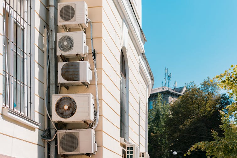
Starting in 1989, the protocol phased out the global production of CFCs by 2010 and prohibited their use in equipment like refrigerators, air-conditioners and insulating foam. This gradual phase-out allowed countries with less established economies time to transition to alternatives and provided funding to help them comply with the protocol’s regulations.

Today, refrigerators and aerosol cans contain gases like propane which, although flammable, does not deplete ozone in Earth’s upper atmosphere when released. However, ozone-friendly alternatives to CFCs in some products, such as certain foams used to insulate fridges, buildings and air-conditioning units, took longer to find. Another set of gases, hydrochlorofluorocarbons (HCFCs), was used as a temporary replacement.

A collection of used refrigerators. — HCFCs can leak to the atmosphere from discarded fridges.
RichardJohnson/Shutterstock

Unfortunately, HCFCs still destroy ozone. The good news is that levels of HCFCs in the atmosphere are now falling and indeed have been since 2021 according to research I led with colleagues. This marks a major milestone in the recovery of Earth’s ozone layer – and offers a rare success story in humanity’s efforts to tackle climate-warming gases too.

HCFCs v CFCs

HCFCs and CFCs have much in common. These similarities are what made the former suitable alternatives.

HCFCs contain chlorine, the chemical element in CFCs that causes these compounds to destroy the ozone layer. HCFCs deplete ozone to a much smaller extent than the CFCs they have replaced – you would have to release around ten times as much HCFC to have a comparable impact on the ozone layer.

But both CFCs and HCFCs are potent greenhouse gases. The most commonly used HCFC, HCFC-22, has a global warming potential of 1,910 times that of carbon dioxide, but only lasts for around 12 years in the atmosphere compared with several centuries for CO₂.

As non-ozone depleting alternatives to HCFCs became available it was decided that amendments to the Montreal protocol were needed to phase HCFCs out. These were agreed in Copenhagen and Beijing in 1992 and 1999 respectively.

This phase-out is still underway. A global target to end most production of HCFCs is set for 2030, with only very minor amounts allowed until 2040.

Turning the corner on a bumpy road

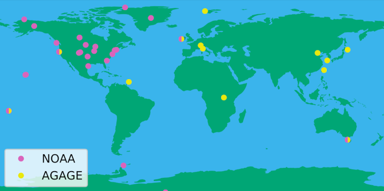
Our findings show that levels of HCFCs in the atmosphere have been falling since 2021 – the first decline since scientists started taking measurements in the late 1970s. This milestone shows the enormous success of the Montreal protocol in not only tackling the original problem of CFCs but also its lesser known and less destructive successor.

Two graphs side by side showing a the climate warming and ozone-destroying influence of HCFCs declining from 2021. — The influence of HCFCs on the atmosphere is set to fall steadily.
Western et al. (2024)/Nature

This is very good news for the ozone layer’s continuing recovery. The most recent scientific prediction, made in 2022, anticipated that HCFC levels would not start falling until 2026.

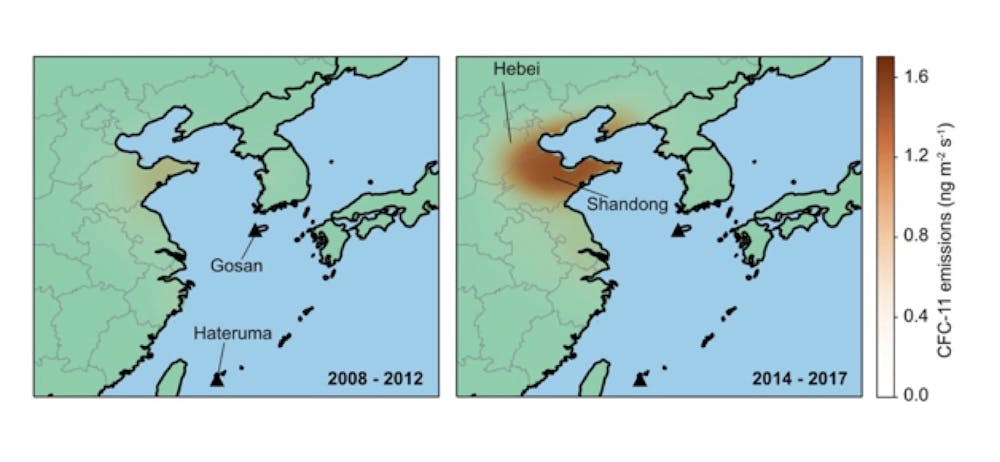
Despite HCFC levels in the atmosphere going in the right direction, not everything has been smooth sailing in the phase-out of ozone-depleting substances. In 2019 a team of scientists, including myself, provided evidence that CFC-11, a common constituent of foam insulation, was still being used in parts of China despite the global ban on production.

The United Nations Environment Programme also reported that HCFCs were illegally produced in 2020 contrary to the phase-down schedule.

In 2023, I and others showed that levels of five more CFCs were increasing in the atmosphere. Rather than illegal production, this increase was more likely the result of a different process: a loophole in the Montreal protocol which allowed CFCs to be produced if they are used to make other substances, such as plastics or non-ozone depleting alternatives to CFCs and HCFCs.

Some HCFCs at very low levels in the atmosphere have also been shown to be increasing or not falling fast enough, despite few or no known uses.

Most of the CFCs and HCFCs still increasing in the atmosphere are released in the production of fluoropolymers – perhaps best known for their application in non-stick frying pans – or hydrofluorocarbons (HFCs).

HFCs are the ozone-friendly alternative that was developed and commercialised in the early 1990s to replace HCFCs, but their role as a potent greenhouse gas means that they are subject to international climate emission reduction treaties such as the Paris agreement and the Kigali amendment to the Montreal protocol.

The next best alternative to climate-warming HFCs is a matter of ongoing discussion. In many applications, it was thought that HFCs would be replaced by hydrofluoroolefins (HFOs), but these have created their own environmental problems in the formation of trifluoroacetic acid which does not break down in the environment and, like other poly- and per-fluorinated substances (PFAS), may pose a risk to human health.

A column of air-conditioning units attached to the exterior of a building. — HFOs enable air-conditioners to use less electricity than competing alternatives.
AndriiKoval/Shutterstock

HFOs are at least more energy-efficient refrigerants than older alternatives like propane, however.

Hope for the future

In discovering this fall in atmospheric levels of HCFCs, I feel like we may be turning the final corner in the global effort to repair the ozone layer. There is still a long way to go before it is back to its original state, but there are now good reasons to be optimistic.

Climate and optimism are two words rarely seen together. But we now know that a small group of potent greenhouse gases called HCFCs have been contributing less and less to climate change since 2021 – and look to set to continue this trend for the foreseeable future.

With policies already in place to phase down HFCs, there is hope that environmental agreements and international cooperation can work in combating climate change.

—————————–

This blog is written by Cabot Institute for the Environment member Dr Luke Western, Research Associate in Atmospheric Science, University of Bristol. This article is republished from The Conversation under a Creative Commons license. Read the original article.

Countries may be under-reporting their greenhouse gas emissions – that’s why accurate monitoring is crucial

Posted on November 16, 2021April 16, 2023 by janet.crompton

Pledges to cut greenhouse gas emissions are very welcome – but accurate monitoring across the globe is crucial if we are to meet targets and combat the devastating consequences of global warming.

During COP26 in Glasgow, many countries have set out their targets to reach net-zero by the middle of this century.

But a serious note of caution was raised in a report in the Washington Post. It revealed that many countries may be under-reporting their emissions, with a gap between actual emissions into the atmosphere and what is being reported to the UN.

This is clearly a problem: if we are uncertain about what we are emitting now, we will not know for certain that we have achieved our emission reduction targets in the future.

Quantifying emissions

Currently, countries must follow international guidelines when it comes to reporting emissions. These reports are based on “bottom-up” methods, in which national emissions are tallied up by combining measures of socioeconomic activity with estimates on the intensity of emissions involved in those activities. For example, if you know how many cows you have in your country and how much methane a typical cow produces, you can estimate the total methane emitted from all the cows.

There are internationally agreed guidelines that specify how this kind of accountancy should be done, and there is a system of cross-checking to ensure that the process is being followed appropriately.

But, according to the Washington Post article, there appear to be some unexpected differences in emissions being reported between similar countries.

The reporting expectations between countries are also considerably different. Developed countries must report detailed, comprehensive reports each year. But, acknowledging the administrative burden of this process, developing countries can currently report much more infrequently.

Plus, there are some noteable gaps in terms of what needs to be reported. For example, the potent greenhouse gases that were responsible for the depletion of the stratospheric ozone layer – such as chlorofluorocarbons (CFCs) – are not included.

A ‘top-down’ view from the atmosphere

To address these issues, scientists have been developing increasingly sophisticated techniques that use atmospheric greenhouse gas observations to keep track of emissions. This “top-down” view measures what is in the atmosphere, and then uses computer models to work backwards to figure out what must have been emitted upwind of the measurements.

To demonstrate the technique, an international team of scientists converged on Glasgow, to observe how carbon dioxide and methane has changed during the COP26 conference.

While this approach cannot provide the level of detail on emission sectors (such as cows, leaks from pipes, fossil fuels or cars) that the “bottom–up” methods attempt, scientists have demonstrated that it can show whether the overall inventory for a particular gas is accurate or not.

The UK was the first country, now one of three along with Switzerland and Australia, to routinely publish top-down emission estimates in its annual National Inventory Report to the United Nations.

A network of five measurement sites around the UK and Ireland continuously monitors the levels of all the main greenhouse gases in the air using tall towers in rural regions.

Emissions are estimated from the measurements using computer models developed by the Met Office. And the results of this work have been extremely enlightening.

In a recent study, we showed that the reported downward trend in the UK’s methane emissions over the last decade is mirrored in the atmospheric data. But a large reported drop before 2010 is not, suggesting the methane emissions were over-estimated earlier in the record.

In another, we found that the UK had been over-estimating emissions of a potent greenhouse gas used in car air conditioners for many years. These studies are discussed with the UK inventory team and used to improve future inventories.

While there is currently no requirement for countries to use top-down methods as part of their reporting, the most recent guidelines and a new World Meteorological Organisation initiative advocate their use as best practice.

If we are to move from only three countries evaluating their emissions in this way, to a global system, there are a number of challenges that we would need to overcome.

Satellites may provide part of the solution. For carbon dioxide and methane, the two most important greenhouse gases, observations from space have been available for more than a decade. The technology has improved dramatically in this time, to the extent that imaging of some individual methane plumes is now possible from orbit.

In 2018, India, which does not have a national monitoring network, used these techniques to include a snapshot of its methane emissions in its report to the UN.

But satellites are unlikely to provide enough information alone.

To move towards a global emissions monitoring system, space-based and surface-based measurements will be required together. The cost to establish ground-based systems such as the UK’s will be somewhere between one million and tens of millions of dollars per country per year.

But that level of funding seems achievable when we consider that billions have been pledged for climate protection initiatives. So, if the outcome is more accurate emissions reporting, and a better understanding of how well we are meeting our emissions targets, such expenditure seems like excellent value for money.

It will be up to the UN and global leaders to ensure that the international systems of measurement and top-down emissions evaluation can be scaled-up to meet the demands of a monitoring system that is fit for purpose. Without robust emissions data from multiple sources, the accuracy of future claims of emission reductions may be called into question.

————————-

This blog is written by Cabot Institute for the Environment member Professor Matt Rigby, Reader in Atmospheric Chemistry, University of Bristol

This article is republished from The Conversation under a Creative Commons license. Read the original article.

How we traced ‘mystery emissions’ of CFCs back to eastern China

Posted on June 5, 2019April 13, 2023 by janet.crompton

Since being universally ratified in the 1980s, the Montreal Protocol – the treaty charged with healing the ozone layer – has been wildly successful in causing large reductions in emissions of ozone depleting substances. Along the way, it has also averted a sizeable amount of global warming, as those same substances are also potent greenhouse gases. No wonder the ozone process is often held up as a model of how the international community could work together to tackle climate change.

However, new research we have published with colleagues in Nature shows that global emissions of the second most abundant ozone-depleting gas, CFC-11, have increased globally since 2013, primarily because of increases in emissions from eastern China. Our results strongly suggest a violation of the Montreal Protocol.

A global ban on the production of CFCs has been in force since 2010, due to their central role in depleting the stratospheric ozone layer, which protects us from the sun’s ultraviolet radiation. Since global restrictions on CFC production and use began to bite, atmospheric scientists had become used to seeing steady or accelerating year-on-year declines in their concentration.

Ozone-depleting gases, measured in the lower atmosphere. Decline since the early 1990s is primarily due to the controls on production under the Montreal Protocol. AGAGE / CSIRO

But bucking the long-term trend, a strange signal began to emerge in 2013: the rate of decline of the second most abundant CFC was slowing. Before it was banned, the gas, CFC-11, was used primarily to make insulating foams. This meant that any remaining emissions should be due to leakage from “banks” of old foams in buildings and refrigerators, which should gradually decline with time.

But in that study published last year, measurements from remote monitoring stations suggested that someone was producing and using CFC-11 again, leading to thousands of tonnes of new emissions to the atmosphere each year. Hints in the data available at the time suggested that eastern Asia accounted for some unknown fraction of the global increase, but it was not clear where exactly these emissions came from.

Growing ‘plumes’ over Korea and Japan

Scientists, including ourselves, immediately began to look for clues from other measurements around the world. Most monitoring stations, primarily in North America and Europe, were consistent with gradually declining emissions in the nearby surrounding regions, as expected.
But all was not quite right at two stations: one on Jeju Island, South Korea, and the other on Hateruma Island, Japan.

These sites showed “spikes” in concentration when plumes of CFC-11 from nearby industrialised regions passed by, and these spikes had got bigger since 2013. The implication was clear: emissions had increased from somewhere nearby.

To further narrow things down, we ran computer models that could use weather data to simulate how pollution plumes travel through the atmosphere.

Atmospheric observations at Gosan and Hateruma monitoring stations showed an increase in CFC-11 emissions from China, primarily from Shandong, Hebei and surrounding provinces. Rigby et al, Author provided

From the simulations and the measured concentrations of CFC-11, it became apparent that a major change had occurred over eastern China. Emissions between 2014 and 2017 were around 7,000 tonnes per year higher than during 2008 to 2012. This represents more than a doubling of emissions from the region, and accounts for at least 40% to 60% of the global increase. In terms of the impact on climate, the new emissions are roughly equivalent to the annual CO₂ emissions of London.

The most plausible explanation for such an increase is that CFC-11 was still being produced, even after the global ban, and on-the-ground investigations by the Environmental Investigations Agency and the New York Times seemed to confirm continued production and use of CFC-11 even in 2018, although they weren’t able to determine how significant it was.

While it’s not known exactly why production and use of CFC-11 apparently restarted in China after the 2010 ban, these reports noted that it may be that some foam producers were not willing to transition to using second generation substitutes (HFCs and other gases, which are not harmful to the ozone layer) as the supply of the first generation substitutes (HCFCs) was becoming restricted for the first time in 2013.

Bigger than the ozone hole

Chinese authorities have said they will “crack-down” on any illegal production. We hope that the new data in our study will help. Ultimately, if China successfully eliminates the new emissions sources, then the long-term negative impact on the ozone layer and climate could be modest, and a megacity-sized amount of CO₂-equivalent emissions would be avoided. But if emissions continue at their current rate, it could undo part of the success of the Montreal Protocol.

The network of global (AGAGE) and US-run (NOAA) monitoring stations. Luke Western, Author provided

While this story demonstrates the critical value of atmospheric monitoring networks, it also highlights a weakness of the current system. As pollutants quickly disperse in the atmosphere, and as there are only so many measurement stations, we were only able to get detailed information on emissions from certain parts of the world.

Therefore, if the major sources of CFC-11 had been a few hundred kilometres further to the west or south in China, or in unmonitored parts of the world, such as India, Russia, South America or most of Africa, the puzzle would remain unsolved. Indeed, there are still parts of the recent global emissions rise that remain unattributed to any specific region.

When governments and policy makers are armed with this atmospheric data, they will be in a much better position to consider effective measures. Without it, detective work is severely hampered.

—————————
This blog is written by Cabot Institute member Dr Matt Rigby, Reader in Atmospheric Chemistry, University of Bristol; Luke Western, Research Associate in Atmospheric Science, University of Bristol, and Steve Montzka, Research Chemist, NOAA ESRL Global Monitoring Division, University of Colorado. This article is republished from The Conversation under a Creative Commons license. Read the original article.

Listen to Matt Rigby talk about CFC emissions on BBC Radio 4’s Inside Science programme.

Antarctica: Why are we here again?

Posted on April 8, 2019April 13, 2023 by janet.crompton

The ship’s roll reaches 19° and everything falls off the desk, nearly followed by me off my chair if it weren’t for an evasive leap to one side. My roommate wakes with a start as the curtains around his bed have flung themselves open. “What are you doing?” he asks, in a confused state. Aside from the fact that everything falling off the desk was the weather’s fault, not mine, his question is a good one.

What are a team of 20 scientists, mostly from the UK, doing out here in the Southern Ocean? Surely there’s somewhere closer to home we could measure the sea. The main aim of this research cruise is to understand the process of deep water formation around Antarctica. First, let me briefly explain what deep water formation is and why it’s important in about 300 words. To understand this, the most important thing to remember is that water becomes denser when it is colder and/or when it is saltier. I think they teach that in GCSE science; if they don’t, they should.

Deep water formation

Antarctica is pretty cold, obviously. Where we are now, the sea temperature is around 1 °C. If we were to go further south or wait until winter, the sea will approach its freezing point of around -2 °C, forming sea ice. That’s a little colder than normal water, which freezes at 0 °C, because the sea is salty. However, when the sea freezes to form sea ice, the salt from the water is not incorporated into the ice – the salt that was in the sea water is left behind, making the remaining water a little bit saltier. As a result, the water close to the sea ice edge is both cold and salty compared to the rest of the world’s oceans, and therefore is denser than most of the rest of the world’s oceans. Dense water sinks below less dense water, and so the deepest water at the bottom of the oceans around the world all comes from around Antarctica.

Sea ice drifting close to the tip of the Antarctic Peninsula

When the water is at the surface of the sea, it can absorb heat and gases, including carbon dioxide, from the atmosphere. When deep water formation occurs, this heat and carbon dioxide can be drawn down into the depths of ocean, where it will stay for 1000 years or so. The research cruise I am on now wants to measure the amount of deep water formation occurring so we can better understand how much heat and carbon dioxide is being taken up by the ocean, which helps understand how much the climate will change in the future with global warming. That’s why we are here, basically, instead of the Bristol Channel.

Chlorofluorocarbons

Our team, based at the University of Exeter, are specifically measuring CFCs in the water. CFCs (chlorofluorocarbons) are manmade gases that were used for many industrial and commercial processes for a few decades before people realised they were destroying ozone in the atmosphere. This was creating a hole in the Earth’s ozone layer in the stratosphere over Antarctica and the Southern Hemisphere. Ozone is important for absorbing some of the Sun’s strong and damaging ultraviolet radiation before it reaches the Earth’s surface. Excessive ultraviolet radiation causes sunburn and skin cancer in humans, so people were concerned about the ozone hole when it was discovered in the 1980s. As a result, all nations of the world agreed the Montreal Protocol to stop producing CFCs that were destroying the ozone layer. Although this was a geopolitical and diplomatic success story, the ozone hole is only slowly showing signs of recovering and some CFCs still seem to be increasing (presumably suggesting some illegal production of them still occurs). However, luckily the ozone hole is no longer getting bigger and it is mostly contained to the very high Southern Hemisphere. Don’t worry, I brought plenty of factor 50 for my pasty Irish skin.

The reason we are measuring CFCs, however, is not actually to understand what they are doing to the ozone layer. We care about CFCs because they are manmade gases that are not naturally found in the atmosphere or ocean. This allows them to be used to trace ocean circulation and processes such as deep water formation. Let me explain how.

Jetsam

Since setting off from the Falklands five weeks ago, we have seen two manmade things: a ship on the horizon and some rusty metal oil barrels floating around amongst a heavy scattering of icebergs. The ship was a fishing boat, not far from the Falklands or Punta Arenas, so was not too surprising. The oil barrels however, were a bit more unexpected. They were floating right in the middle of the Weddell Sea, almost as far from civilisation as they could be. There were at least four of them, however they weren’t lashed together like some sort of raft made by Tom Hanks, they were all floating individually within a few hours steam of each other.

Oil barrel floating in the Weddell Sea, originally dumped around 6,000 km away (image credit: Hugh Venables, BAS)

The most curious thing about these barrels, however, is that when we were able to zoom in on a photo taken of one with a camera with a good telephoto lens, we could see their origin. They had writing and the branding from Operation Deepfreeze, a US mission to set up an Antarctic base in the Ross Sea in the 1950s. After initially being surprised at seeing any litter in the pristine Southern Ocean, we had to question how these barrels got here. The Ross Sea is on the entire other side of the Antarctic continent, around 6,000 km away by sea.

The Operation Deepfreeze base was built on the Ross Ice Shelf. This is thick ice that has flown out from the glaciers on land to create an area the size of France floating over the Ross Sea. Although this ice is very thick and reasonably slow moving, it is not permanent and does break off from time to time to form huge icebergs. The same process has formed some icebergs that have made the news recently, including one berg a quarter of the size of Wales and a potential berg break off that is threatening to take the British Antarctic Survey’s Halley research station with it. Well, presumably the old dumping ground from Operation Deepfreeze has at some stage broken off from the Ross Ice Shelf, floated halfway around the Southern Ocean carried by the Antarctic Circumpolar Current and been taken into the Weddell Sea gyre, where it melted and broke up, scattering all the rubbish into the Weddell Sea.

Just like these oil barrels can be used to trace how the ocean’s surface currents circulate (a similar story involves a spilt shipping container of rubber ducks in the Pacific Ocean in 1992), looking at where manmade gases such as CFCs end up in the deep ocean can tell us how the deep water formation takes water from the surface to depth. To measure the CFCs, we first take samples using a probe known as a CTD (which stands for Conductivity Temperature Depth). This probe has 24 bottles on it as well as instruments for measuring of salinity, temperature and other water properties. The probe is lowered to the bottom of the ocean (which around here can be more than 6 km deep) and as it is brought back up to the surface, the 24 bottles are closed at different depths. When the CTD arrives back on the ship’s deck, we then have samples of water from 24 depths through the ocean at that particular location. Over the course of the cruise, we will be carrying out around 100 CTDs.

Sampling using the CTD (lowered by winch off the side of the ship) continues morning, noon and night, meaning we work 12 hour shifts

With the water brought up in the bottles, our team takes a 500 ml sample from each and we store them in a walk-in fridge on the ship. We then analyse one sample at a time, which takes about 20 minutes using a custom-built machine that strips all the gases out of the water and calculates the amount of CFCs it contains. This setup for measuring CFCs is in its own portable lab, built in a shipping container that it strapped onto the aft deck of the James Clark Ross. While it’s pretty time-consuming running 100 CTDs with 24 bottles each taking 20 minutes (I calculate that to be more than 33 days of continually running the machine, assuming no delays) at least we have a good view from our container out over the wildlife and icebergs of the Southern Ocean.

Our CFC lab inside a shipping container, strapped onto the aft deck, as we sail by the South Orkney Islands

Other science

Besides our team measuring CFCs, other scientists are also using the water from the CTD to analyse oxygen isotopes, nutrient content, pH and microbes. When the CTD comes on deck, there is usually a bit of a mad scramble as everyone gets water for their own analysis, with a strict pecking order as who gets to take their water first. For maximum inconvenience, usually the CTD comes up just before dinner or lunch, just to make sampling that little bit more frantic.

Taking water samples for analysis from the 24 bottles on the CTD once it is back on deck (image credit: Charel Wohl, PML)

As well as measuring water from depth using the CTD, other scientists on the ship also continually measure the air and surface sea water as we sail. The air measurements, taken from the very front of the ship so not to get contaminated by exhaust or air conditioning fumes, must be measuring some of the cleanest air in the world. It’s pretty nice to stand up there and breathe it in, although it’s often accompanied by a blizzard of snow and biting wind, which makes the experience slightly less enjoyable.

We also have deployed some floats that will continue to measure the salinity and temperature of the sea here for the next five years or so. Using a gas bladder, these floats can adjust their density so they rise and sink through the ocean, measuring continually as they go. Every time these floats get back to the surface, they send their data back via a satellite connection. Although they don’t measure as much stuff as the scientists on the ship (for example, they don’t measure CFCs), they will be here all year round so keep making measurements through the winter. The ship on the other hand will have to retreat from the sea ice before the winter sets in, in case we end up repeating Shackleton’s antics with the Endurance. Which is fine with me because, interesting as it is, I don’t really fancy a further 6 months down here in the dark.

A float being deployed, which will continue to make measurements through the winter and for years after we leave

——————————————-
This blog is part of a blog series from Antarctica by Alan Kennedy-Asser, who has recently completed his PhD at the University of Bristol. This blog has been republished with kind permission from Alan. View the original blog. You can follow Alan on Twitter @EzekielBoom.

Alan Kennedy-Asser

Read part one of Alan’s Antarctica blog series – Antarctica: Ship life
Read part two of Alan’s Antarctica blog series – Antarctica: Why are we here again?
Read part three of Alan’s Antarcica blog series: Antarctica: Looking back

Antarctica: Ship life

Posted on March 25, 2019April 13, 2023 by janet.crompton

The RRS James Clark Ross docked in the Falkland Islands

Blinking blurry eyes, I crack open the curtains and gaze out into the bright light of a new day. A hulking white and blue iceberg gazes back at me. Even after a broken night’s sleep being shunted from one side of my bunk to the other as the ship bounces through swell, that still makes a rewarding start to each day. Through an unexpected turn of events, I’ve found myself on the British Antarctic Survey’s RRS James Clark Ross, on a seven-week long research cruise helping researchers from the University of Exeter take samples and measure CFCs in the Weddell Sea. Having just handed in my PhD thesis – after four years of studying and researching Antarctic climate and hearing the question “do you get to go to Antarctica?” countless times – the opportunity to help out on this cruise was too good an opportunity to pass up. Life on a ship gives you plenty of time to think (and write), but I promise to keep these musings brief in three posts: ship life; the science and why we’re here; and how the real thing compares to a PhD.
—————————————-
This is my first experience of life on a ship. Previously, my most extensive experience of boat life was the eight hours on the Stena Line from Liverpool to Belfast, so I shall use that as my reference frame. Stena Line regularly ask you to fill out feedback forms and rate your experience to have the chance to win back the cost of your trip, so I shall do the same here (although as usual I don’t expect to win anything).

How did you find the booking procedure?

Stena Line have a fast and efficient website for making and managing bookings. Signing up for the research cruise was also pretty straight forward, although that was likely aided by me having done a PhD in Antarctic-related science and knowing someone at the British Antarctic Survey (BAS) who forwarded me the advert. I emailed the lead scientist from Exeter saying I was interested, we had a chat on Skype then I had to confirm that my PhD supervisors at Bristol were happy for me to go.

Generally, however, beyond that point there was a bit more faff than booking the Stena Line. BAS require quite a few forms filling out, some of which require a bit more homework, including passing a medical examination and a sea survival course. The authentic personal sea survival certificate had to be presented on getting on the boat before sailing. In contrast, the Stena Line rarely even ask for ID (although I suppose this might change after Brexit).

Stena Line: 5/5
James Clark Ross: 3/5

How did you find the check-in procedure?

The check-in for the Stena is remarkably simple, and as mentioned they rarely even ask for ID. Getting onto the James Clark Ross was logistically more complicated, requiring flights from Heathrow to Madrid, Madrid to Santiago in Chile, and Santiago to Punta Arenas. Although this journey took more than 24 hours, I still preferred it to driving in the rain up the M5 and M6 from Bristol, as I got free food and could watch films. Punta Arenas is also nicer than Birkenhead and I found the language barrier easier to overcome in Chile (Scouse can be very confusing at times).

Stena Line: 3/5
James Clark Ross: 4/5

Exploring the Magellanic forest above Punta Arenas

How did you find the cabins (if applicable)?

Getting a cabin on the Stena Line is not necessary, particularly if travelling during the day time sailing. The last time I travelled on the night time crossing, however, the cabin was not overly satisfactory with uncomfortable beds, an unclean bathroom and a broken soap dispenser. Stena customer services subsequently refunded the cost of the cabin. On the James Clark Ross, the cabins are slightly smaller than the Stena Line, however, there is ample storage space, the beds are pretty comfortable and there are privacy curtains for each bunk, which is good when you are on slightly different work shifts to your roommate. The biggest complaint about the James Clark Ross is that it makes many strange noises and rocks a lot more in the heavy weather, which can keep you up a lot of the night. These noises include a high-pitched wail which is either the stabiliser system or sirens luring us to our watery graves. The latter seems more likely.

Stena Line: 1/5
James Clark Ross: 3/5

How did you find the food onboard?

The Stena’s Met Grill is renowned for its fried breakfast and hearty lunch and dinner menu. The portion sizes are good, however, the prices are also a bit steep. On the James Clark Ross, three square meals a day are available (including midnight dinner service for those on night shifts), with lunch and dinner both offering 3+ courses. Because of how my shift patterns work out, it doesn’t make sense to get up for breakfast, so I just eat a 3-course lunch and dinner each day. Remarkably, over 4 weeks since we left, there is still fresh fruit and some salad on the go. The variety has been good, and they also have included some of the classics off the Stena Line menu, including fish and chips (most Fridays), curry (every Saturday) and Swedish meatballs. Although I have also had Swedish meatballs on the Stena, I have never tried authentic (Ikea) Swedish meatballs to know which is closer to the real deal.

Stena Line: 4/5
James Clark Ross: 5/5

How did you find the onboard shopping?

The shop onboard the Stena Line is pretty awful. They sell head phones if you forgot yours, which is about the only thing I have ever bought from it. They also sell some magazines and over-priced toys in case you didn’t realise the crossing was 8 hours and find yourself going slightly insane. The shop on the James Clark Ross, called the bond, is stocked with James Clark Ross branded clothing, toiletries, chocolate bars and some odds and ends like postcards and plaques. Unfortunately, as the ship is nearing the end of its working life for BAS, being replaced next year by the RRS Sir David Attenborough (of Boaty McBoatface fame), none of the branded clothing is being restocked. That means the only things that are left are in sizes XXL or age 7-8, neither of which are much use to me.

Stena Line: 1/5
James Clark Ross: 1/5

How did you find the onboard entertainment and facilities?

Both ships have a bar. The James Clark Ross bar is extremely cheap, however, many of the beers are about six months past their best before dates, which can result in ‘bowel roulette’ the following day. A worthwhile sacrifice if you’re unemployed like me. The lounge area is remarkably similar between both boats and is comfortable enough. The internet connection is much better on the Stena, although they possibly harvest your personal data in the process of providing it. On the James Clark Ross, they have to commit some of the internet to facilitate the science (boring), so the bandwidth for personal connections is not as strong.

Besides the gambling machines, the Stena Line’s main attraction is the cinema, which can be good if they have a decent film being shown. On the James Clark Ross, although they do not have a dedicated cinema room, they have a huge selection of DVDs and an endless supply of films available on people’s laptops which can all be put through a projector. There are also loads of board games and a few musical instruments onboard too, which are nice to have a jam on and facilitated a St Patrick’s Day gig and ceilidh dance. Although the James Clark Ross has a greater range of entertainment available, the Stena Line only has to keep you amused for 8 hours, not 7 weeks, so this one is a tight run context. Luckily when you have to work 12 hour shifts, you don’t have much time for entertainment.

Stena Line: 3/5
James Clark Ross: 4/5

St Patrick’s Day decorations in the bar

Would you recommend this crossing to a friend?

Usually my answer to this is ‘yes’ for the Stena Line. It’s a handy way of getting to England from Belfast, saving the drive through North Wales and up from Dublin. Admittedly there’s not much to see in the Irish Sea except the odd shearwater and the Isle of Mann, but generally the crossing is smooth because of the size of the ship (around 185m long) even when the weather is bad. On the James Clark Ross, the research cruise route very much agrees with the old saying ‘The adventure is in the journey, not the destination’. We are analysing a transect through the Southern Ocean and Weddell Sea and end at 57.5°S, 30°E, which is precisely in the middle of nowhere (go ahead and look it up on Google Maps). Although we don’t end anywhere in particular, the route has been spectacular at times: we’ve sailed past a number of sub-Antarctic islands, countless colossal icebergs, seen penguins on land, in the sea and on ice, had dolphins, fin whales, and humpbacks right by the ship (the latter breaching dramatically at times) and had regular, effortless fly-bys from wandering albatrosses and other seabirds great and small. The weather has been mixed and as the ship is 100m long it feels the swell a bit more than the Stena, however, the seas so far have been much more merciful than I had expected.

Humpbacks taking a breath, Coronation Island, South Orkneys

As exciting as it is to see the Isle of Mann and the Mourne Mountains, on the whole, I would say Antarctica just about tops the Irish Sea. Sorry Stena Line. Although, for health and safety reasons I’m sure the crew of the Stena Mersey are happy enough to not have to dodge all of these icebergs.

Stena Line: 4/5
James Clark Ross: 5/5

—————————–
This blog is part of a blog series from Antarctica by Alan Kennedy-Asser, who has recently completed his PhD at the University of Bristol. This blog has been republished with kind permission from Alan. View the original blog. You can follow Alan on Twitter @EzekielBoom.

Alan Kennedy-Asser

Independent verification of the UK’s greenhouse gas report: holding the Government to account

Posted on November 7, 2016April 6, 2023 by janet.crompton

In the early hours of October 15th, negotiators from over 170 countries finalised a legally binding accord, designed to counter the effects of climate change by way of phasing down emissions of Hydrofluorocarbons (HFCs). These gases, introduced to replace the ozone-depleting CFCs and HCFCs for which the original Montreal Protocol was drafted, are typically used as coolants in air-conditioning systems. Unfortunately, like their predecessors, they are potent greenhouse gases, whose climate forcing effect per molecule is often many thousands of times greater than carbon dioxide.

The Kigali deal, named after the Rwandan city in which it was struck, is a compromise between rich countries, whose phase-out plan will begin as early as 2019, and poorer nations, for many of whom the relief of air-conditioning has only just become available. India, for instance, will not make its first 10% emissions cut until 2032.

Delegates celebrate the finalisation of the Kigali deal. Credit: COP 22

When the deal was finally completed, there was much celebration and relief. Against the ironic drone of several large air-conditioning units, brought in to maintain a comfortable temperature on a stifling Rwandan night, US Secretary of State John Kerry labelled the deal ‘a monumental step forward’.

However, as with the much lauded Paris Agreement, the success of this landmark piece of legislation will rely heavily on accountability. Each nation reports its greenhouse gas emissions, including HFCs, to the United Nations Framework Convention on Climate Change (UNFCCC). It is from these reports that a nation’s progress in cutting emissions can be assessed.

Here at the University of Bristol’s Atmospheric Chemistry Research Group (ACRG), we use atmospheric measurements of these greenhouse gases, in combination with an atmospheric transport model, to independently estimate emissions. Recently, we have used such an approach to estimate emissions of HFC-134a, the most abundant HFC in the global atmosphere. Observations of this gas were taken from the Mace Head Observatory, which can be found on the rugged West Coast of Ireland.

When we compared our emission estimates with those the UK government reported to the UNFCCC, a significant discrepancy was observed; between 1995 and 2012, the UNFCCC numbers are consistently double those derived independently.

The Mace Head observatory is ideally positioned to intercept air mass from the UK and Europe. Credit – University of Bristol

Via collaboration with DECC (Department of Energy and Climate Change), the government body that was previously responsible for the construction of the UKs annual emissions report, we were granted access to the model used to estimate HFC-134a emissions. Analysis of this model uncovered a number of assumptions made about the UK’s HFC markets, which in practice did not add up. Our work has led to a reassessment of the HFC-134a inventory by the government, and a subsequent lowering of the reported emission totals in the 2016 report.

In the wake of the Kigali and Paris agreements, both of which will require accurate reporting of emissions, our work is amongst the first examples of how independent verification can directly influence inventory totals. However, this study represents just the tip of the iceberg. Across the Kyoto ‘basket’ of gases determined to have an adverse effect on climate, inconsistencies between reporting methods are common place. A more concerted effort is therefore required to harmonise inventory reports with independent studies.

In countries such as the UK, where networks capable of measuring these gases already exist, the focus will be on improving the accuracy and reducing the uncertainty of our emission estimates; a step which will likely involve the addition of new sites, new instrumentation and significant investment.

Perhaps more importantly, these methods of independent verification must now be extended to regions where such infrastructure does not currently exist. Emissions from many of these countries are anticipated to rise sharply in the coming years, but are poorly monitored.

In July, researchers from the ACRG returned from Northern India, after two months studying greenhouse gas emissions from the FAAM research aircraft.

The Atmospheric Research Aircraft from the Facility for
Airborne Atmospheric Measurements (FAAM), established by NERC and the Met Office as a facility for the
UK atmospheric science community. Credit – FAAM

The utilisation of different data platforms is likely to play an essential role in enhancing the global network of greenhouse gas observations. It is the responsibility of the research community to ensure continued growth of the measurement network, and improve the availability of independent emission estimates required to verify the success (or otherwise) of climate legislation.

This blog was written for the Policy Bristol Blog by Dan Say, PhD student, Atmospheric Chemistry
Research Group, School of Chemistry, University of Bristol.

Deep impact – the plastic on the seafloor; the carbon in the air

Posted on June 9, 2014April 14, 2023 by janet.crompton

We live in a geological age defined by human activity. We live during a time when the landscape of the earth has been transformed by men, its surface paved and cut, its vegetation manipulated, transported and ultimately replaced. A time when the chemical composition of the atmosphere, the rivers and the oceans has been changed – in some ways that are unique for the past million years and in other ways that are unprecedented in Earth history. In many ways, this time is defined not only by our impact on nature but by the redefinition of what it means to be human.

From a certain distance and perspective, the transformation of our planet can be considered beautiful. At night, the Earth viewed from space is a testament to the ubiquitous presence of the human species: cities across the planet glow with fierce intensity but so do villages in Africa and towns in the Midwest; the spotlights of Argentine fishing boats, drawing anchovies to the surface, illuminate the SW Atlantic Ocean; and the flames of flared gas from fracked oil fields cause otherwise vacant tracts of North Dakota to burn as bright as metropolises.

Environmental debates are a fascinating, sometimes frustrating collision of disparate ideas, derived from different experiences, ideologies and perspectives. And we learn even from those with whom we disagree. However, one perspective perpetually bemuses and perplexes me: the idea that it is impossible that man could so transform this vast planet. Of course, we can pollute an estuary, cause the Cuyahoga River to catch fire, turn Victorian London black or foul the air of our contemporary cities. We can turn the Great Plains into cornfields or into dust bowls, the rainforest into palm oil plantations, swamplands into cities and lowlands into nations. But these are local. Can we really be changing our oceans, our atmosphere, our Earth that much?

Such doubts underly the statements of, for example, UKIP Energy Spokesman Roger Helmer:

‘The theory of man-made climate change is unproven and implausible’.

It is a statement characterised by a breathless dismissal of scientific evidence but also an astonishingly naive view of man’s capacity to impact our planet.

There are places on Earth where the direct evidence of human intervention is small. There are places where the dominance of nature is vast and exhilarating and awe-inspiring. And across the planet, few places are entirely immune from reminders – whether they be earthquakes or volcanoes, tsunamis or hurricanes – that nature is vast and powerful.

But the Earth of the 21st century is a planet shaped by humans.

*********

A powerful example of humanity’s impact on our planet is our Plastic Ocean. We generate nearly 300 billion tons of plastic per year, much of it escaping recycling and much of that escaping the landfill and entering our oceans. One of the most striking manifestations of this is the vast trash vortex in the Northern Pacific Gyre. The size of the vortex depends on assumptions of concentration and is somewhat dependent on methodology, but estimates range from 700 thousand square kilometres to more than 15 million square kilometres. The latter estimate represents nearly 10% of the entire Pacific Ocean. Much of the plastic in the trash vortex – and throughout our oceans – occurs as fine particles invisible to the eye. But they are there and they are apparently ubiquitous, with concentrations in the trash vortex reaching 5.1 kg per square km*. That’s equivalent to about 200 1L bottles. Dissolved. Invisible to the eye. But present and dictating the chemistry of the ocean.

More recently, colleagues at Plymouth, Southampton and elsewhere illustrated the widespread occurrence of rubbish, mainly plastic, on the ocean floor. Their findings did not surprise deep sea biologists nor geologists; we have been observing our litter in these supposedly pristine settings since some of the first trips to the abyss.

My first submersible dive was on the Nautile, a French vessel that was part of a joint Dutch-French expedition to mud volcanoes and associated methane seeps in the Mediterranean Sea. An unfortunate combination of working practice, choppy autumn seas and sulfidic sediments had made me seasick for most of the research expedition, such that my chance to dive to the seafloor was particularly therapeutic. The calm of the deep sea, as soon as we dipped below the wave base, was a moment of profound physical and emotional peace. As we sank into the depths, the light faded and all that remained was the very rare fish and marine snow – the gently sinking detritus of life produced in the light-bathed surface ocean.

As you descend, you enter a realm few humans had seen…. For a given dive, for a given locale, it is likely that no human has preceded you.

Mud volcanoes form for a variety of reasons, but in the Mediterranean region they are associated with the tectonic interactions of the European and African continents. This leads to the pressurised extrusion of slurry from several km below the bottom of the sea, along mud diapirs and onto the seafloor. They are commonly associated with methane seeps; in fact a focus of our expedition was to examine the microbes and wider deep sea communities that thrive when this methane is exposed to oxidants at the seafloor – a topic for another essay. In parts of the Mediterranean Sea, they are associated with salty brines, partially derived from the great salt deposits that formed in a partly evaporated ocean about five and a half million years ago.

And all of these factors together create an undersea landscape of indescribable beauty.
On these mud volcanoes are small patches, about 20 cm wide, where methane escapes to the seafloor. There, methane bubbles from the mud or is capped by thick black, rubbery mats of microorganisms. Ringing these mats are fields of molluscs, bouquets of tube worms, great concrete slabs of calcium carbonate or white rims of sulphide and the bacteria thriving on it. Streaming from these seeps, down the contours of the mud cones, are ribbons of ultra-dense, hypersaline water. The rivulets merge into streams and then into great deep sea rivers. Like a photonegative of low-density oil slicking upon the water’s surface, these are white, high-density brines flowing along the seafloor. Across the Mediterranean Sea, they pool into beautiful ponds and in a few very special cases, form great brine lakes.

And two kilometres below the seafloor, where humans have yet to venture our rubbish has already established colonies. Plastic bottles float at the surface of these lakes; aluminium cans lie in the mud amongst the microbial mats; between those thick slabs of calcium carbonate sprout colonies of tube worms and the occasional plastic bag.

Image from Nautile Dive to the Mediterranean seafloor. Shown are carbonate crusts that form where methane has escaped to the seafloor as well as tube worms thriving on the chemical energy available in such settings. Plastic debris has been circled in the upper right corner.

We have produced as much plastic in the past decade as we have in the entirety of the preceding human history. But the human impact is not new. On our very first dive, we observed a magnificent amphora, presumably of ancient Greek or Roman origin and nearly a metre across, half buried in the mud.

*********

Today the human footprint is ubiquitous. Nearly 40% of the world’s land is used for agriculture – and over 70% of the land in the UK. Another 3% of the land is urbanised. A quarter of arable land has already been degraded.

There are outstanding contradictions and non-intuitive patterns that emerge from a deeper understanding of this modified planet. Pollinators are more diverse in England’s cities than they are in our rural countryside. One of the most haunting nature preserves on our planet is the Demilitarized Zone between North and South Korea – fraught with landmines but free from humans, wildlife now dominates. And of course, although global warming will cause vast challenges over the coming centuries, that is largely due to one human impact (greenhouse gas emissions) intersecting with another (our cities in vulnerable, low-lying areas and our borders and poverty preventing migration from harm). And on longer timescales, we have likely spared our descendants of 10,000 years from now the hassle of dealing with another Ice Age.

Glyptodon, source Wikipedia

But there can be no doubt or misunderstanding – we have markedly changed the chemical composition of our atmosphere. Carbon dioxide levels are higher than they have been for the past 800,000 years, perhaps the last 3 million years. It is likely that the last time the Earth’s atmosphere contained this much carbon dioxide, glyptodons, armadillo-like creatures the size of cars, roamed the American West, and hominids were only beginning the first nervous evolutionary steps towards what would eventually become man. Methane concentrations are three times higher than they were before the agricultural and industrial revolutions. Also higher are the concentrations of nitrous oxides. And certain chlorofluorcarbons did not even exist on this planet until we made them.

The manner in which we have changed our planet has – at least until now – allowed us to thrive, created prosperity and transformed lives in ways that would have astonished those from only a few generations in the past. It is too soon to say whether our collective impact has been or will be, on the whole, either ‘good’ or ‘bad’ for either the planet or those of us who live upon it. It will perhaps never be possible to define such a complex range of impacts in simple black and white terms. But there is no doubt that our impact has been vast, ubiquitous and pervasive. And it is dangerous to underestimate even momentarily our tremendous capacity to change our planet at even greater rates and in even more profound ways in the future.

*Moore, C.J; Moore, S.L; Leecaster, M.K;
Weisberg, S.B (2001). “A Comparison of Plastic and Plankton in the North
Pacific Central Gyre”. Marine
Pollution Bulletin 42 (12): 1297–300. doi:10.1016/S0025-326X(01)00114-X. PMID 11827116.

This blog is by Prof Rich Pancost, Director of the Cabot Institute.

Prof Rich Pancost

‘New’ man-made gases: Ozone crisis or hoax?

Posted on March 14, 2014April 19, 2023 by janet.crompton

Image by PiccoloNamek (English wikipedia)
[GFDL (www.gnu.org/copyleft/fdl.html),
via Wikimedia Commons

You may have noticed a story reported on widely recently on the discovery of 4 ‘new’ man-made ozone-depleting gases. This follows the publication of a study in the journal Nature Geoscience on the first measurements of these gases, their abundances in the atmosphere and estimated global emission rates. Responses to the reporting of this publication have ranged from the Daily Mail’s “Ozone Crisis” to the inevitable internet-based diatribe of “any research from UEA is clearly made up” in various comment sections. So just how concerned should we be about the emissions of these four gases?

Chlorofluorcarbons (CFCs)

The reason we care about CFCs is because they deplete ozone high up in the atmosphere, potentially exposing humans to harmful UV rays. Oh, they also happen to be extremely potent greenhouse gases, with each molecule of a CFC being equivalent to 1000s of molecules of CO₂, and they sit around in the atmosphere for 10s or 100s of years before being removed. Basically they’re pretty bad, and sure they might have been great refrigerants and aerosol propellants but at what cost?

The production of CFCs has now to all intents and purposes ceased, although that doesn’t mean that emissions have completely stopped; various banks of these gases exist in fridges for example. These might leak during use or when destroyed. So it’s not entirely surprising to read that this study has found that various CFCs are still being released.

Newly measured

In fact the reason this paper is important is more to do with the fact that these gases have never before been measured. Many of the media articles seem to lead with the fact these are ‘new’ ozone-depleting gases, which is a little misleading. They’re not new; they’ve been around for decades, only nobody has been able to measure them in the atmosphere before. Why’s that you might ask? Well much of it is to do with just how small their concentrations are in the atmosphere.

The fact of the matter is that the concentrations of these gases (CFC-112, CFC-112a, CFC-113a, HCFC-133a) are tiny. All four have atmospheric mixing ratios of less than 1 part per trillion (ppt). In other words, if you could isolate a trillion molecules of air (1 x 10¹²) then not even one of them would be one of these ’new’ CFCs. By contrast CO₂ in the atmosphere has a mixing ratio of hundreds of parts per million.

Compare these newly measured gases to the major CFCs (CFC-11, CFC-12, CFC-113) whose current atmospheric concentrations are hundreds if not thousands of times greater. Even though emissions of these major CFCs are now close to zero they will still be around in the atmosphere at these elevated concentrations for decades to come. This is shown in the plot below taken from the AGAGE network measurements of CFC-12. Although the concentration has reached a peak it will take at least one hundred years for levels to get back down to pre-1980 levels, with the current mixing ratio still over 500 ppt.

Plot taken from the AGAGE network measurements of CFC-12

So emissions of these newly measured gases would have to really pick up for a sustained period of time to add significantly to the ozone-depleting effect of what is already in the atmosphere. To say the measurement of these compounds has created some sort of ozone crisis is therefore a gross exaggeration. That’s not to say that this work was a waste of time; it’s vital that we know about these compounds and their atmospheric abundance so we can ensure their contribution to ozone depletion remains negligible.

Other factors influencing ozone recovery

There are other potentially more important causes for concern as well. Hydrochlorofluorocarbons (HCFCs) were introduced as replacements for CFCs but also contribute to ozone depletion, albeit in a less effective way. Although these are also being phased out many of these will have a greater impact on the recovery of the ozone ‘hole’ than these newly measured species. Just a few months ago the United Nations Environment Programme (UNEP) released a report saying another gas, Nitrous Oxide (N₂O), is now considered to be the biggest threat to the ozone layer over the next 50 years. Not to mention that one of the impacts of a rise in global surface temperatures could be a slowing in ozone hole recovery. There’s a genuinely interesting (honest!) explanation for why that is which I will cover in another blog.

The point is that there are lots of factors which affect the Earth’s ozone layer. Studies like the one recently published in Nature Geoscience are vital for our understanding of what the recent and current atmospheric composition is like. It might not be a problem now, but surely the key to looking after our planet, and ourselves, is to prevent things from becoming problematic in future. If we can take steps to find out where these emissions are coming from and why some of them are increasing then measures could be put in place to limit their future influence on ozone recovery.

This blog is written by Mark Lunt, Atmospheric Chemistry Reseach Group, Cabot Institute, University of Bristol, .

Mark Lunt

35 years monitoring the changing composition of our atmosphere

Posted on November 4, 2013April 20, 2023 by janet.crompton

I work on an experiment that began when the Bee Gees’ Stayin’ Alive was at the top of the charts. The project is called AGAGE, the Advanced Global Atmospheric Gases Experiment, and I’m here in Boston, Massachusetts celebrating its 35-year anniversary. AGAGE began life in 1978 as the Atmospheric Lifetimes Experiment, ALE, and has been making high-frequency, high-precision measurements of atmospheric trace gases ever since.

At the time of its inception, the world had suddenly become aware of the potential dangers associated with CFCs (chlorofluorocarbons). What were previously thought to be harmless refrigerants and aerosol propellants were found to have a damaging influence on stratospheric ozone, which protects us from harmful ultraviolet radiation. The discovery of this ozone-depletion process was made by Mario Molina and F. Sherwood Rowland, for which they, and Paul Crutzen, won the Nobel Prize in Chemistry in 1995. However, Molina and Rowland were not sure how long CFCs would persist in the atmosphere, and so ALE, under the leadership of Prof. Ron Prinn (MIT) and collaborators around the world, was devised to test whether we’d be burdened with CFCs in our atmosphere for years, decades or centuries.

Fig 1. The AGAGE network

ALE monitored the concentration of CFCs, and other ozone depleting substances, at five sites chosen for their relatively “unpolluted” air (including the west coast of Ireland station which is now run by Prof. Simon O’Doherty here at the University of Bristol). The idea was that if we could measure the increasing concentration of these gases in the air, then, when combined with estimates of the global emission rate, we would be able to determine how rapidly natural processes in the atmosphere were removing them.

Fig 2. Mace Head station on the West coast of Ireland

Thanks in part to these measurements, we now know that CFCs will only be removed from the atmosphere over tens to hundreds of years, meaning that the recovery of stratospheric ozone and the famous ozone “hole” will take several generations. However, over the years, ALE, and now AGAGE, have identified a more positive story relating to atmospheric CFCs: the effectiveness of international agreements to limit gas emissions.

The Montreal Protocol on Substances that Deplete the Ozone Layer was agreed upon after the problems associated with CFCs were recognised. It was agreed that CFC use would be phased-out in developed countries first, and developing countries after a delay of a few years. The effects were seen very rapidly. For some of the shorter-lived compounds, such as methyl chloroform (shown in the figure), AGAGE measurements show that global concentrations began to drop within 5 years of the 1987 ratification of the Protocol.

Figure 3. Concentrations of methyl chloroform, a substance banned under the Montreal Protocol, measured at four AGAGE stations.

Over time, the focus of AGAGE has shifted. As the most severe consequences of stratospheric ozone depletion look like they’ve been avoided, we’re now more acutely aware of the impact of “greenhouse” gases on the Earth’s climate. In response, AGAGE has developed new techniques that can measure over 40 compounds that are warming the surface of the planet. These measurements are showing some remarkable things, such as the rapid growth of HFCs, which are replacements for CFCs that have an unfortunate global-warming side effect, or the strange fluctuations in atmospheric methane concentrations, which looked like they’d plateaued in 1999, but are now growing rapidly again.

The meeting of AGAGE team members this year has been a reminder of how important this type of meticulous long-term monitoring is. It’s also a great example of international scientific collaboration, with representatives attending from the USA, UK, South Korea, Australia, Switzerland, Norway and Italy. Without the remarkable record that these scientists have compiled, we’d be much less informed about the changing composition of the atmosphere, more unsure about the lifetimes of CFCs and other ozone depleting substances, and unclear as to the exact concentrations and emissions rates of some potent greenhouse gases. I’m looking forward to the insights we’ll gain from the next 35 years of AGAGE measurements!This blog was written by Dr Matt Rigby, Atmospheric Chemistry Research Group, University of Bristol.

Matt Rigby