Hydrological modelling and pizza making: why doesn’t mine look like the one in the picture?

Is this a question that you have asked yourself after following a recipe, for instance, to make pizza?

You have used the same ingredients and followed all the steps and still the result doesn’t look like the one in the picture…

Don’t worry: you are not alone! This is a common issue, and not only in cooking, but also in hydrological sciences, and in particular in hydrological modelling.

Most hydrological modelling studies are difficult to reproduce, even if one has access to the code and the data (Hutton et al., 2016). But why is this?

In this blog post, we will try to answer this question by using an analogy with pizza making.

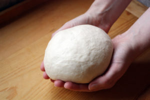
Let’s imagine that we have a recipe together with all the ingredients to make pizza. Our aim is to make a pizza that looks like the one in the picture of the recipe.

This is a bit like someone wanting to reproduce the results reported in a scientific paper about a hydrological “rainfall-runoff” model. There, one would need to download the historical data (rainfall, temperature and river flows) and the model code used by the authors of the study.

However, in the same way as the recipe and the ingredients are just the start of the pizza making process, having the input data and the model code is only the start of the modelling process.

To get the pizza shown in the picture of the recipe, we first need to work the ingredients, i.e. knead the dough, proof and bake. And to get the simulated river flows shown in the study, we need to ‘work’ the data and the model code, i.e. do the model calibration, evaluation and final simulation.

Using the pizza making analogy, these are the correspondences between pizza making and hydrological modelling:

Pizza making                         Hydrological modelling

kitchen and cooking tools computer and software

ingredients                         historical data and computer code for model simulation

recipe                                 modelling process as described in a scientific paper or in a computer                                                         script / workflow

Step 1: Putting the ingredients together

Dough kneading

So, let’s start making the pizza. According to the recipe, we need to mix well the ingredients to get a dough and then we need to knead it. Kneading basically consists of pushing and stretching the dough many times and it can be done either manually or automatically (using a stand mixer).

The purpose of kneading is to develop the gluten proteins that create the structure and strength in the dough, and that allow for the trapping of gases and the rising of the dough.The recipe recommends using a stand mixer for the kneading, however if we don’t have one, we can do it manually.

The recipe says to knead until the dough is elastic and looks silky and soft. We then knead the dough until it looks like the one in the photo shown in the recipe.

Model calibration

Now, let’s start the modelling process. If the paper does not report the values of the model parameters, we can determine them through model calibration. Model calibration is a mathematical process that aims to tailor a general hydrological model to a particular basin. It involves running the model many times under different combinations of the parameter values, until one is found that matches well the flow records available for that basin. Similarly to kneading, model calibration can be manual, i.e. the modeller changes manually the values of the model parameters trying to find a combination that captures the patterns in the observed flows (Figure 1), or it can be automatic, i.e. a computer algorithm is used to search for the best combination of parameter values more quickly and comprehensively.

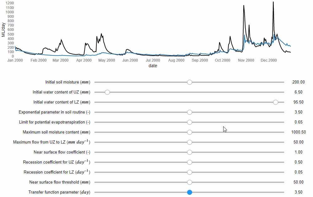
Figure 1 Manual model calibration. The river flows predicted by the model are represented by the blue line and the observed river flows by the black line (source: iRONS toolbox)

According to the study, the authors used an algorithm implemented in an open source software for the calibration. We can download and use the same software. However, if any error occurs and we cannot install it, we could decide to calibrate the model manually. According to the study, the Nash-Sutcliffe efficiency (NSE) function was used as numerical criteria to evaluate the calibration obtaining a value of 0.82 out of 1. We then do the manual calibration until we obtain NSE = 0.82.

(source: iRONS toolbox)

Step 2: Checking our work

Dough proofing

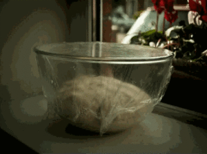
In pizza making, this step is called proofing or fermentation. In this stage, we place the dough somewhere warm, for example close to a heater, and let it rise. According to the recipe, the proofing will end after 3 hours or when the dough has doubled its volume.

The volume is important because it gives us an idea of how strong the dough is and how active the yeast is, and hence if the dough is ready for baking. We let our dough rise for 3 hours and we check. We find out that actually it has almost tripled in size… “even better!” we think.

Model evaluation

In hydrological modelling, this stage consists of running the model using the parameter values obtained by the calibration but now under a different set of temperature and rainfall records. If the differences between estimated and observed flows are still low, then our calibrated model is able to predict river flows under meteorological conditions different from the one to which it was calibrated. This makes us more confident that it will work well also under future meteorological conditions. According to the study, the evaluation gave a NSE = 0.78. We then run our calibrated model fed by the evaluation data and we get a NSE = 0.80… “even better!” we think.

Step 3: Delivering the product!

Pizza baking

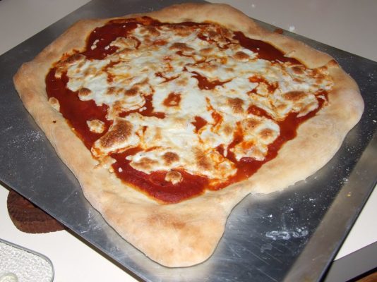
Finally, we are ready to shape the dough, add the toppings and bake our pizza. According to the recipe, we should shape the dough into a round and thin pie. This takes some time as our dough keeps breaking when stretched, but we finally manage to make it into a kind of rounded shape. We then add the toppings and bake our pizza.

Ten minutes later we take the pizza out of the oven and… it looks completely different from the one in the picture of the recipe! … but at least it looks like a pizza…

(Source: flickr.com)

River flow simulation

And finally, after calibrating and evaluating our model, we are ready to use it to simulate recreate the same river flow predictions as shown in the results of the paper. In that study, they forced the model with seasonal forecasts of rainfall and temperature that are available from the website of the European Centre for Medium-range Weather Forecasts (ECMWF).

Downloading the forecasts takes some time because we need to write two scripts, one to download the data and one to pre-process them to be suitable for our basin (so called “bias correction”). After a few hours we are ready to run the simulation and… it looks completely different from the hydrograph shown in the study! … but at least it looks like a hydrograph…

Why we never get the exact same result?

Here are some possible explanations for our inability to exactly reproduce pizzas or modelling results:

  • We may have not kneaded the dough enough or kneaded it too much; or we may have thought that the dough was ready when it wasn’t. Similarly, in modelling, we may have stopped the calibration process too early or too late (so called “over-fitting” of the data).
  • The recipe does not provide sufficient information on how to test the dough; for example, it does not say how wet or elastic the dough should be after kneading. Similarly, in modelling, a paper may not provide sufficient information about model testing as, for instance, the model performance for different variables and different metrics.
  • We don’t have the same cooking tools as those used by the recipe’s authors; for example, we don’t have the same brand of the stand mixer or the oven. Similarly, in modelling we may use a different hardware or operating system, which means calculations may differ due to different machine precision or slightly different versions of the same software tools/dependencies.
  • Small changes in the pizza making process, such as ingredients quantities, temperature and humidity, can lead to significant changes in the final result, particularly because some processes, such as kneading, are very sensitive to small changes in conditions. Similarly, small changes in the modelling process, such as in the model setup or pre-processing of the data, can lead to rather different results.

In conclusion…

Setting up a hydrological model involves the use of different software packages, which often exist in different versions, and requires many adjustments and choices to tailor the model to a specific place. So how do we achieve reproducibility in practice? Sharing code and data is essential, but often is not enough. Sufficient information should also be provided to understand what the model code does, and whether it does it correctly when used by others. This may sound like a big task, but the good news is that we have increasingly powerful tools to efficiently develop rich and interactive documentation. And some of these tools, such as R Markdown or Jupyter Notebooks, and the online platforms that support them such as Binder, enable us not only to share data and code but also the full computational environment in which results are produced – so that others have access not only to our recipes but can directly cook in our kitchen.

—————————

This blog has been reposted with kind permission from the authors, Cabot Institute for the Environment members Dr Andres Peñuela, Dr Valentina Noacco and Dr Francesca Pianosi. View the original post on the EGU blog site.

Andres Peñuela is a Research Associate in the Water and Environmental Engineering research group at the University of Bristol. His main research interest is the development and application of models and tools to improve our understanding on the hydrological and human-impacted processes affecting water resources and water systems and to support sustainable management and knowledge transfer


Valentina Noacco is a Senior Research Associate in the Water and Environmental Engineering research group at the University of Bristol. Her main research interest is the development of tools and workflows to transfer sensitivity analysis methods and knowledge to industrial practitioners. This knowledge transfer aims at improving the consideration of uncertainty in mathematical models used in industry


Francesca Pianosi is a Senior Lecturer in Water and Environmental Engineering at the University of Bristol. Her expertise is in the application of mathematical modelling to hydrology and water systems. Her current research mainly focuses on two areas: modelling and multi-objective optimisation of water resource systems, and uncertainty and sensitivity analysis of mathematical models.


What global threats should we be most worried about in 2019?

The Cambridge Global Risk Index for 2019 was presented on 4 December 2018 in the imposing building of Willis Towers Watson in London. The launch event aimed to provide an overview of new and rising risk challenges to allow governments and companies to understand the economic implications of various risks. My interest, as a Knowledge Exchange Fellow working with the (re)insurance sector to better capture the uncertainties embedded in its models, was to find out how the index could help insurance companies to better quantify risks.

The presentation started with the Cambridge Centre for Risk Studies giving an introduction on which major world threats are included in the index, followed by a panel discussion on corporate innovation and ideation.

The Cambridge Global Risk Index quantifies the impact future catastrophic events (be they natural or man-made) would have on the world’s economy, by looking at the GDP at risk in the most prominent cities in the world (GDP@Risk). The Index includes 22 threats in five categories: natural disasters and climate; financial, economics and trade; geopolitics and security; human pandemic and plant epidemic; and technology and space.

Global Risk Index 2019 Threat Rankings (Cambridge Global Risk Index 2019 Executive Summary)

The GDP@Risk for 2019 for the 279 cities studied, which represents 41% of the global GDP, has been estimated to be $577bn or 1.57% of the GDP of 2019. The GDP@Risk has increased since last year by more than 5%, which was caused by both an increase in GDP globally and a rise in the chances of losses from a cyber attack and other threats to richer economies. Risk is becoming ever more interconnected due to cascading threats, such as natural hazards and climate events triggering power outages, geopolitical tensions triggering cyber attacks sponsored by states, conflicts worsening human epidemics, and trade wars triggering sovereign crises, which in turn caused social unrest.

Nonetheless, the GDP@Risk can be reduced  by making cities more resilient, that is improving the ability of a city to be prepared for a shock and to recover from it.  For example, if the worst off 100 cities in the world would be as prepared as the top cities, they could reduce their exposure to risk by around 30%, which shows the importance of investing in resilience and recoverability. This is a measure of what the insurance industry calls the “protection gap”, how much could be earned from investments to improve the preparedness and resilience of a city to shocks. How fast a city recovers depends on the ability to access capital, to reconstruct and repair factories, houses and infrastructure, to restore consumers’ confidence and to reduce the length of business interruption.

Global Risk Index 2019 Growth by Sub-Category ($, bn) (Cambridge Global Risk Index 2019 Executive Summary)

Natural catastrophe and climate

After a 2017 with the second highest losses due to natural disasters, 2018 saw several record-breaking natural catastrophes as well. This year we have experienced events from magnitude 7.5 earthquakes and tsunami in Indonesia, which caused more then 3000 deaths, to the second highest number of tropical cyclones active in a month, from Typhoon Mangkhut in the Philippines, to Japan’s strongest storm in the last two decades. Hurricanes have beaten records too, with hurricane Florence in North Carolina becoming the 2nd wettest hurricane on record, which caused $10 bn losses, and hurricane Michael in Florida reaching the greatest wind speeds ever recorded, which caused $15 bn losses.

Floods in 2018 caused heavy death tolls in Japan and south India, with 225 and 500 fatalities respectively, the former showing the weakness of an ageing city infrastructure, while the latter raising criticism on poor forecasting and management of water resources. Droughts raged in South Africa, Australia, Argentina, Uruguay and Italy reducing harvests, while wildfires in California were the largest on record, which caused $20 bn losses. Extreme events have made it to weather events too, with extreme heatwaves, as the hottest summer in the UK, comparable to the one of 1976, and the heatwave in Japan which hospitalised 35,000 people, as well as with extreme freeze, as the “Beast from the East” in the UK which caused losses estimated at $1 billion per day.

Extreme events are becoming ever more frequent due to climate change, with the next few years expected to be anomalously warm, even on top of the regular climate change. This hints that the rising trend in losses due to natural catastrophe and climate is not due to stop.

Devastation from the cyclone in Tonga, 2018.

Finance, economics and trade

Market crash is the number one threat for 2019, which could cause more than $100 billion in losses. Nonetheless global financial stability is improving due to increased regulation, but risk appetite has increased as well due to positive growth prospects and low interest rates, which increases financial vulnerabilities. Trade disputes between the US and China and the US and Europe are disrupting the global supply chains. The proportion of GDP@Risk has increased in Italy due to policy uncertainty and increased sovereign risks, while in countries such as Greece, Cyprus and Portugal sovereign debt risks have decreased following restructuring of their debt and country level credit rating upgrades.

Geopolitics and security

The risk from geopolitics and security worldwide has remained relatively similar compared to last year, with roughly the same countries being in conflict as in 2017. Iran’s proxy presence remains in conflicts in Yemen, Iraq, Israel, Syria and Lebanon, while social unrest has increased risk in Yemen, Nicaragua, Venezuela, Argentina, Iraq and South Africa. The conflict in Yemen has caused the world’s worst humanitarian crises in 2018, with more than 2 million displaced, with food shortages and malnutrition causing cholera outbreak. The total expected loss from this category is similar to the one from financial, economic and trade risk.

Technology and space

Technology and space is the category with the lowest expected GDP at risk. Nevertheless, the risk has increased over recent years, with cyber attacks becoming ever more frequent due to the internationalisation of cyber threat, the increasing size and cost of data breaches, the continued disruption from DDoS attacks, the threat to critical infrastructure, and its continuous evolution and sophistication. Cyber attacks have climbed one level in the ranking this year, assuring the 6th overall position. In 2017 the WannaCry ransomware attacks affected 300,000 computers across 150 countries disrupting critical city infrastructure, such as healthcare, railways, banks, telecoms and energy companies, while NotPetya produced quarterly losses of $300 million for various companies. The standstill faced by the city of Atlanta when all its computers were locked due to a ransomware attack in March caused £2.6 million to be spent, and another $9.5 million are expected. This attack highlighted the breath of potential disruption, with energy, nuclear, water, aviation and manufacturing infrastructure at risk. Moreover 66% of companies are estimated to have experienced a supply chain attack, costing on average $1.1 million per attack. In response to these threats, countries are increasing their spending on cyber offensive capability, with the UK spending hundreds of millions of pounds. Power outage, nuclear accident and solar storm are not at the top of the threats ranking globally, but solar storms could cause over $4bn of GDP@Risk in North American cities, due to their position in northern latitudes, leaving 20-40 million people without power.


Health and humanity

The greatest threat to humanity according to the UN is anti-microbial resistance, with areas in the world already developing strains of malaria and tuberculosis resistant to all available medicines. It is expected that over the next 35 years 300 million people will die prematurely due to drug resistance, decreasing the world’s GDP between 2 and 3.5% in 2050. Major epidemics have remained largely constrained in the same areas as last year, and are fuelled by climate and geopolitical crises which aggravates hygiene and public health, such as the Yemen and Somalia cholera outbreaks. Plant epidemics have not increased, with the ongoing problems of Panama disease in bananas, coffee and wheat rust, and the xylella fastidiosa still affecting olive plants in southern Europe.

Corporate innovation and ideation discussion

The panel discussed the importance of the Cambridge Global Risk Index to prepare companies for future threats. For example, for insurance companies including the index in their management of risk would allow them to be better prepared and more profitable. I found the words of Francine Stevens, director of Innovation at Hiscox, particularly inspiring. She talked about how the sheer volume of research produced is often too large to be digested by practitioners, and how workshops might help to bring people with similar interests together to pull out what are the most exciting topics and challenges to work on. As a Knowledge Exchange Fellow myself, this strikes a familiar chord, as it is my job to transfer research to the insurance sector and I have first-hand experience on the importance of adopting a common language and identifying how industry uptakes new research and methods.

Francine has also talked about the importance of collaboration between companies, a particularly sensitive topic in the highly competitive insurance sector. This topic emerged also at the insurance conference held by the Oasis Loss Modelling Framework in September, where the discussion touched on how non-competitive collaborations could bring the sector forward by avoiding duplication. Francine’s final drop of wisdom was about the importance of diversity to drive innovation, and how having a group of smart people with diverse backgrounds often delivers better results than a group of high-achievers with the same background. And this again sounded very familiar!

————————————-
This blog is written by Cabot Institute member Dr Valentina Noacco, a NERC Knowledge Exchange Fellow and a Senior Research Associate at the University of Bristol Department of Civil Engineering. Her research looks at improving the understanding and consideration of uncertainty in the (re)insurance industry. This blog reports material with the consent of the Cambridge Centre for Risk Studies and is available online at https://www.jbs.cam.ac.uk/faculty-research/centres/risk/news-events/events/2018/cambridge-global-risk-index-2019-launch-event/.

Dr Valentina Noacco